Distributed NumPy on a Cluster with Dask Arrays

This work is supported by Continuum Analytics the XDATA Program and the Data Driven Discovery Initiative from the Moore Foundation

This page includes embedded large profiles. It may look better on the actual site rather than through syndicated pages like planet.python and it may take a while to load on non-broadband connections (total size is around 20MB)

Summary

We analyze a stack of images in parallel with NumPy arrays distributed across a cluster of machines on Amazon’s EC2 with Dask array. This is a model application shared among many image analysis groups ranging from satellite imagery to bio-medical applications. We go through a series of common operations:

1. Inspect a sample of images locally with Scikit Image
2. Construct a distributed Dask.array around all of our images
3. Process and re-center images with Numba
4. Transpose data to get a time-series for every pixel, compute FFTs

This last step is quite fun. Even if you skim through the rest of this article I recommend checking out the last section.

Inspect Dataset

I asked a colleague at the US National Institutes for Health (NIH) for a biggish imaging dataset. He came back with the following message:

Electron microscopy may be generating the biggest ndarray datasets in the field - terabytes regularly. Neuroscience needs EM to see connections between neurons, because the critical features of neural synapses (connections) are below the diffraction limit of light microscopes. This type of research has been called “connectomics”. Many groups are looking at machine vision approaches to follow small neuron parts from one slice to the next.

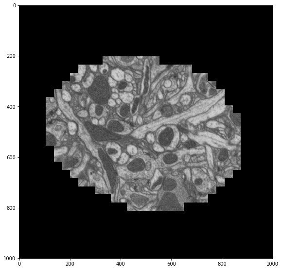
This data is from drosophila: http://emdata.janelia.org/. Here is an example 2d slice of the data http://emdata.janelia.org/api/node/bf1/grayscale/raw/xy/2000_2000/1800_2300_5000.

import skimage.io
import matplotlib.pyplot as plt

sample = skimage.io.imread('http://emdata.janelia.org/api/node/bf1/grayscale/raw/xy/2000_2000/1800_2300_5000'
skimage.io.imshow(sample)

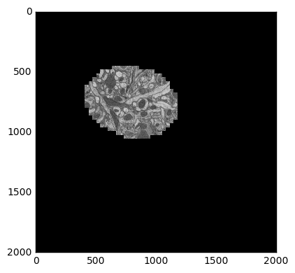
The last number in the URL is an index into a large stack of about 10000 images. We can change that number to get different slices through our 3D dataset.

samples = [skimage.io.imread('http://emdata.janelia.org/api/node/bf1/grayscale/raw/xy/2000_2000/1800_2300_%d' % i)
    for i in [1000, 2000, 3000, 4000, 5000, 6000, 7000, 8000, 9000]]

fig, axarr = plt.subplots(1, 9, sharex=True, sharey=True, figsize=(24, 2.5))
for i, sample in enumerate(samples):
    axarr[i].imshow(sample, cmap='gray')

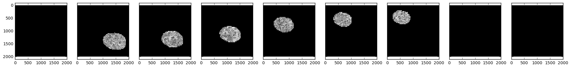
We see that our field of interest wanders across the frame over time and drops off in the beginning and at the end.

Create a Distributed Array

Even though our data is spread across many files, we still want to think of it as a single logical 3D array. We know how to get any particular 2D slice of that array using Scikit-image. Now we’re going to use Dask.array to stitch all of those Scikit-image calls into a single distributed array.

import dask.array as da
from dask import delayed

imread = delayed(skimage.io.imread, pure=True)  # Lazy version of imread

urls = ['http://emdata.janelia.org/api/node/bf1/grayscale/raw/xy/2000_2000/1800_2300_%d' % i
        for i in range(10000)]  # A list of our URLs

lazy_values = [imread(url) for url in urls]     # Lazily evaluate imread on each url

arrays = [da.from_delayed(lazy_value,           # Construct a small Dask array
                          dtype=sample.dtype,   # for every lazy value
                          shape=sample.shape)
          for lazy_value in lazy_values]

stack = da.stack(arrays, axis=0)                # Stack all small Dask arrays into one

>>> stack
dask.array<shape=(10000, 2000, 2000), dtype=uint8, chunksize=(1, 2000, 2000)>

>>> stack = stack.rechunk((20, 2000, 2000))     # combine chunks to reduce overhead
>>> stack
dask.array<shape=(10000, 2000, 2000), dtype=uint8, chunksize=(20, 2000, 2000)>

So here we’ve constructed a lazy Dask.array from 10 000 delayed calls to skimage.io.imread. We haven’t done any actual work yet, we’ve just constructed a parallel array that knows how to get any particular slice of data by downloading the right image if necessary. This gives us a full NumPy-like abstraction on top of all of these remote images. For example we can now download a particular image just by slicing our Dask array.

>>> stack[5000, :, :].compute()
array([[0, 0, 0, ..., 0, 0, 0],
       [0, 0, 0, ..., 0, 0, 0],
       [0, 0, 0, ..., 0, 0, 0],
       ...,
       [0, 0, 0, ..., 0, 0, 0],
       [0, 0, 0, ..., 0, 0, 0],
       [0, 0, 0, ..., 0, 0, 0]], dtype=uint8)

>>> stack[5000, :, :].mean().compute()
11.49902425

However we probably don’t want to operate too much further without connecting to a cluster. That way we can just download all of the images once into distributed RAM and start doing some real computations. I happen to have ten m4.2xlarges on Amazon’s EC2 (8 cores, 30GB RAM each) running Dask workers. So we’ll connect to those.

from dask.distributed import Client, progress
client = Client('schdeduler-address:8786')

>>> client
<Client: scheduler="scheduler-address:8786" processes=10 cores=80>

I’ve replaced the actual address of my scheduler (something like 54.183.180.153 with `scheduler-address. Let’s go ahead and bring in all of our images, persisting the array into concrete data in memory.

stack = client.persist(stack)

This starts downloads of our 10 000 images across our 10 workers. When this completes we have 10 000 NumPy arrays spread around on our cluster, coordinated by our single logical Dask array. This takes a while, about five minutes. We’re mostly network bound here (Janelia’s servers are not co-located with our compute nodes). Here is a parallel profile of the computation as an interactive Bokeh plot.

There will be a few of these profile plots throughout the blogpost, so you might want to familiarize yoursel with them now. Every horizontal rectangle in this plot corresponds to a single Python function running somewhere in our cluster over time. Because we called skimage.io.imread 10 000 times there are 10 000 purple rectangles. Their position along the y-axis denotes which of the 80 cores in our cluster that they ran on and their position along the x-axis denotes their start and stop times. You can hover over each rectangle (function) for more information on what kind of task it was, how long it took, etc.. In the image below, purple rectangles are skimage.io.imread calls and red rectangles are data transfer between workers in our cluster. Click the magnifying glass icons in the upper right of the image to enable zooming tools.

Now that we have persisted our Dask array in memory our data is based on hundreds of concrete in-memory NumPy arrays across the cluster, rather than based on hundreds of lazy scikit-image calls. Now we can do all sorts of fun distributed array computations more quickly.

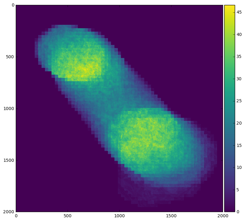
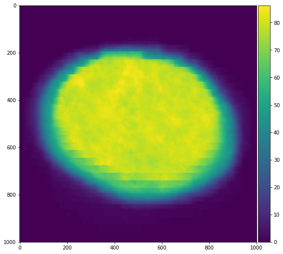
For example we can easily see our field of interest move across the frame by averaging across time:

skimage.io.imshow(stack.mean(axis=0).compute())

Or we can see when the field of interest is actually present within the frame by averaging across x and y

plt.plot(stack.mean(axis=[1, 2]).compute())

By looking at the profile plots for each case we can see that averaging over time involves much more inter-node communication, which can be quite expensive in this case.

Recenter Images with Numba

In order to remove the spatial offset across time we’re going to compute a centroid for each slice and then crop the image around that center. I looked up centroids in the Scikit-Image docs and came across a function that did way more than what I was looking for, so I just quickly coded up a solution in Pure Python and then JIT-ed it with Numba (which makes this run at C-speeds).

from numba import jit

@jit(nogil=True)
def centroid(im):
    n, m = im.shape
    total_x = 0
    total_y = 0
    total = 0
    for i in range(n):
        for j in range(m):
            total += im[i, j]
            total_x += i * im[i, j]
            total_y += j * im[i, j]

    if total > 0:
        total_x /= total
        total_y /= total
    return total_x, total_y

>>> centroid(sample)  # this takes around 9ms
(748.7325324581344, 802.4893005160851)

def recenter(im):
    x, y = centroid(im.squeeze())
    x, y = int(x), int(y)
    if x < 500:
        x = 500
    if y < 500:
        y = 500
    if x > 1500:
        x = 1500
    if y > 1500:
        y = 1500

    return im[..., x-500:x+500, y-500:y+500]

plt.figure(figsize=(8, 8))
skimage.io.imshow(recenter(sample))

Now we map this function across our distributed array.

import numpy as np
def recenter_block(block):
    """ Recenter a short stack of images """
    return np.stack([recenter(block[i]) for i in range(block.shape[0])])

recentered = stack.map_blocks(recenter,
                              chunks=(20, 1000, 1000),  # chunk size changes
                              dtype=a.dtype)
recentered = client.persist(recentered)

This profile provides a good opportunity to talk about a scheduling failure; things went a bit wrong here. Towards the beginning we quickly recenter several images (Numba is fast), taking around 300-400ms for each block of twenty images. However as some workers finish all of their allotted tasks, the scheduler erroneously starts to load balance, moving images from busy workers to idle workers. Unfortunately the network at this time appeared to be much slower than expected and so the move + compute elsewhere strategy ended up being much slower than just letting the busy workers finish their work. The scheduler keeps track of expected compute times and transfer times precisely to avoid mistakes like this one. These sorts of issues are rare, but do occur on occasion.

We check our work by averaging our re-centered images across time and displaying that to the screen. We see that our images are better centered with each other as expected.

skimage.io.imshow(recentered.mean(axis=0))

This shows how easy it is to create fast in-memory code with Numba and then scale it out with Dask.array. The two projects complement each other nicely, giving us near-optimal performance with intuitive code across a cluster.

Rechunk to Time Series by Pixel

We’re now going to rearrange our data from being partitioned by time slice, to being partitioned by pixel. This will allow us to run computations like Fast Fourier Transforms (FFTs) on each time series efficiently. Switching the chunk pattern back and forth like this is generally a very difficult operation for distributed arrays because every slice of the array contributes to every time-series. We have N-squared communication.

This analysis may not be appropriate for this data (we won’t learn any useful science from doing this), but it represents a very frequently asked question, so I wanted to include it.

Currently our Dask array has chunkshape (20, 1000, 1000), meaning that our data is collected into 500 NumPy arrays across the cluster, each of size (20, 1000, 1000).

>>> recentered
dask.array<shape=(10000, 1000, 1000), dtype=uint8, chunksize=(20, 1000, 1000)>

But we want to change this shape so that the chunks cover the entire first axis. We want all data for any particular pixel to be in the same NumPy array, not spread across hundreds of different NumPy arrays. We could solve this by rechunking so that each pixel is its own block like the following:

>>> rechunked = recentered.rechunk((10000, 1, 1))

However this would result in one million chunks (there are one million pixels) which will result in a bit of scheduling overhead. Instead we’ll collect our time-series into 10 x 10 groups of one hundred pixels. This will help us to reduce overhead.

>>> # rechunked = recentered.rechunk((10000, 1, 1))  # Too many chunks
>>> rechunked = recentered.rechunk((10000, 10, 10))  # Use larger chunks

Now we compute the FFT of each pixel, take the absolute value and square to get the power spectrum. Finally to conserve space we’ll down-grade the dtype to float32 (our original data is only 8-bit anyway).

x = da.fft.fft(rechunked, axis=0)
power = abs(x ** 2).astype('float32')

power = client.persist(power, optimize_graph=False)

This is a fun profile to inspect; it includes both the rechunking and the subsequent FFTs. We’ve included a real-time trace during execution, the full profile, as well as some diagnostics plots from a single worker. These plots total up to around 20MB. I sincerely apologize to those without broadband access.

Here is a real time plot of the computation finishing over time:

And here is a single interactive plot of the entire computation after it completes. Zoom with the tools in the upper right. Hover over rectangles to get more information. Remember that red is communication.

Screenshots of the diagnostic dashboard of a single worker during this computation.

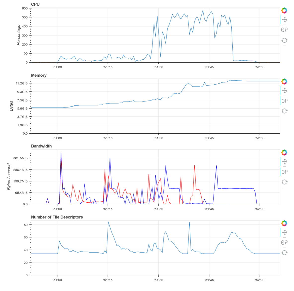
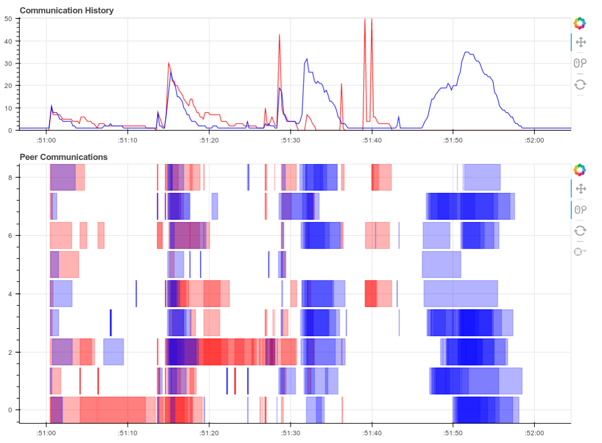
This computation starts with a lot of communication while we rechunk and realign our data (recent optimizations here by Antoine Pitrou in dask #417). Then we transition into doing thousands of small FFTs and other arithmetic operations. All of the plots above show a nice transition from heavy communication to heavy processing with some overlap each way (once some complex blocks are available we get to start overlapping communication and computation). Inter-worker communication was around 100-300 MB/s (typical for Amazon’s EC2) and CPU load remained high. We’re using our hardware.

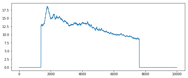
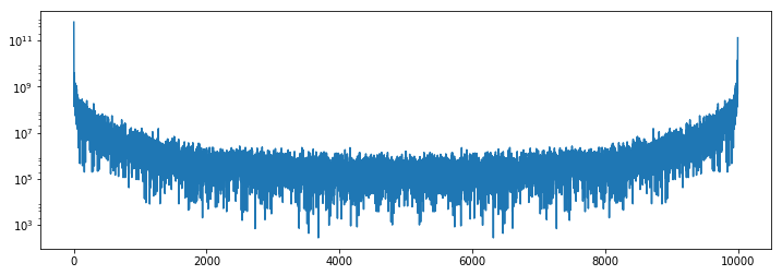
Finally we can inspect the results. We see that the power spectrum is very boring in the corner, and has typical activity towards the center of the image.

plt.semilogy(1 + power[:, 0, 0].compute())

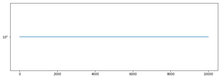
plt.semilogy(1 + power[:, 500, 500].compute())

Final Thoughts

This blogpost showed a non-trivial image processing workflow, emphasizing the following points:

1. Construct a Dask array from lazy SKImage calls.
2. Use NumPy syntax with Dask.array to aggregate distributed data across a cluster.
3. Build a centroid function with Numba. Use Numba and Dask together to clean up an image stack.
4. Rechunk to facilitate time-series operations. Perform FFTs.

Hopefully this example has components that look similar to what you want to do with your data on your hardware. We would love to see more applications like this out there in the wild.

What we could have done better

As always with all computationally focused blogposts we’ll include a section on what went wrong and what we could have done better with more time.

1. Communication is too expensive: Interworker communications that should be taking 200ms are taking up to 10 or 20 seconds. We need to take a closer look at our communications pipeline (which normally performs just fine on other computations) to see if something is acting up. Disucssion here dask/distributed #776 and early work here dask/distributed #810.
2. Faulty Load balancing: We discovered a case where our load-balancing heuristics misbehaved, incorrectly moving data between workers when it would have been better to let everything alone. This is likely due to the oddly low bandwidth issues observed above.
3. Loading from disk blocks network I/O: While doing this we discovered an issue where loading large amounts of data from disk can block workers from responding to network requests (dask/distributed #774)
4. Larger datasets: It would be fun to try this on a much larger dataset to see how the solutions here scale.