Data Proximate Computation on a Dask Cluster Distributed Between Data Centres
By Duncan McGregor (Met Office), Mike Grant (EUMETSAT), Richard Care (Met Office)
This work is a joint venture between the Met Office and the European Weather Cloud, which is a partnership of ECMWF and EUMETSAT.
Summary
We have devised a technique for creating a Dask cluster where worker nodes are hosted in different data centres, connected by a mesh VPN that allows the scheduler and workers to communicate and exchange results.
A novel (ab)use of Dask resources allows us to run data processing tasks on the workers in the cluster closest to the source data, so that communication between data centres is minimised. If combined with zarr to give access to huge hyper-cube datasets in object storage, we believe that the technique could realise the potential of data-proximate distributed computing in the Cloud.
Introduction
The UK Met Office has been carrying out a study into data-proximate computing in collaboration with the European Weather Cloud. We identified Dask as a key technology, but whilst existing Dask techniques focus on parallel computation in a single data centre, we looked to extend this to computation across data centres. This way, when the data required is hosted in multiple locations, tasks can be run where the data is rather than copying it.
Dask worker nodes exchange data chunks over a network, coordinated by a scheduler. There is an assumption that all nodes are freely able to communicate, which is not generally true across data centres due to firewalls, NAT, etc, so a truly distributed approach has to solve this problem. In addition, it has to manage data transfer efficiently, because moving data chunks between data centres is much more costly than between workers in the same cloud.
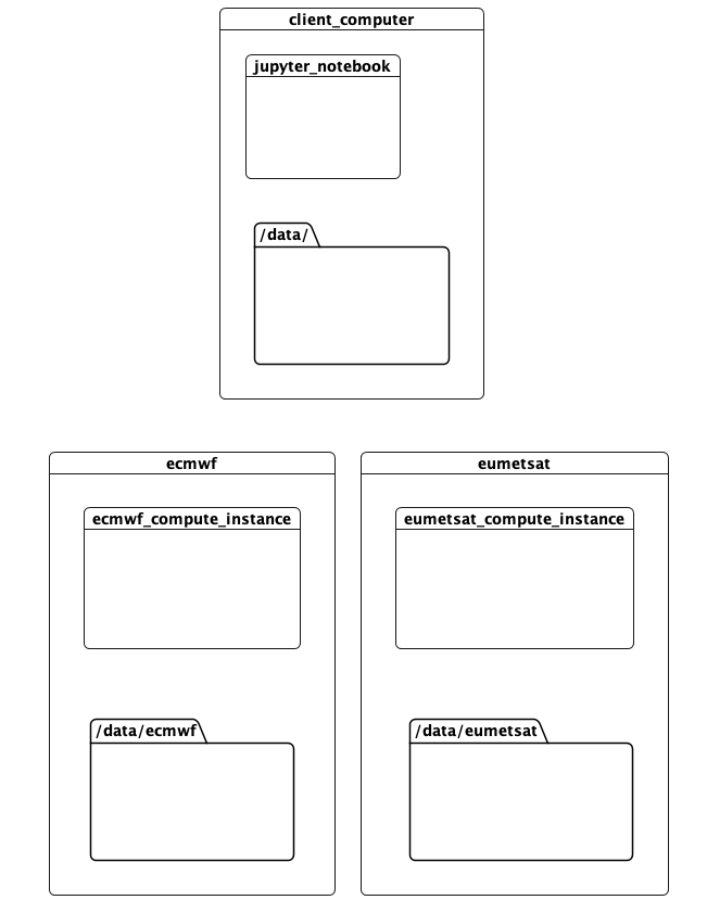
This notebook documents a running proof-of-concept that addresses these problems. It runs a computation in 3 locations:
- This computer, where the client and scheduler are running. This was run on AWS during development.
- The ECMWF data centre. This has compute resources, and hosts data containing predictions.
- The EUMETSAT data centre, with compute resources and data on observations
from IPython.display import Image
Image(filename="images/datacentres.png") # this because GitHub doesn't render markup images in private repos
The idea is that tasks accessing data available in a location should be run there. Meanwhile the computation can be defined, invoked, and the results rendered, elsewhere. All this with minimal hinting to the computation as to how this should be done.
Setup
First some imports and conveniences
import os
from time import sleep
import dask
from dask.distributed import Client
from dask.distributed import performance_report, get_task_stream
from dask_worker_pools import pool, propagate_pools
import pytest
import ipytest
import xarray
import matplotlib.pyplot as plt
from orgs import my_org
from tree import tree

ipytest.autoconfig()
In this case we are using a control plane IPv4 WireGuard network on 10.8.0.0/24 to set up the cluster - this is not a necessity, but simplifies this proof of concept. WireGuard peers are running on ECMWF and EUMETSAT machines already, but we have to start one here:
!./start-wg.sh
4: mo-aws-ec2: <POINTOPOINT,NOARP,UP,LOWER_UP> mtu 8921 qdisc noqueue state UNKNOWN group default qlen 1000
    link/none
    inet 10.8.0.3/24 scope global mo-aws-ec2
       valid_lft forever preferred_lft forever
We have worker machines configured in both ECMWF and EUMETSAT, one in each. They are accessible on the control plane network as
ecmwf_host='10.8.0.4'
%env ECMWF_HOST=$ecmwf_host
eumetsat_host='10.8.0.2'
%env EUMETSAT_HOST=$eumetsat_host
env: ECMWF_HOST=10.8.0.4
env: EUMETSAT_HOST=10.8.0.2
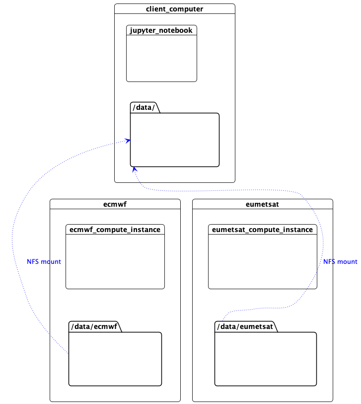
Mount the Data
This machine needs access to the data files over the network in order to read NetCDF metadata. The workers are sharing their data with NFS, so we mount them here. (In this proof of concept, the control plane network is used for NFS, but the data plane network could equally be used, or a more appropriate technology such as zarr accessing object storage.)
%%bash
sudo ./data-reset.sh

mkdir -p /data/ecmwf
mkdir -p /data/eumetsat
sudo mount $ECMWF_HOST:/data/ecmwf /data/ecmwf
sudo mount $EUMETSAT_HOST:/eumetsatdata/ /data/eumetsat
Image(filename="images/datacentres-data.png")
Access to Data
For this demonstration, we have two large data files that we want to process. On ECMWF we have predictions in /data/ecmwf/000490262cdd067721a34112963bcaa2b44860ab.nc. Workers running in ECMWF can see the file
!ssh -i ~/.ssh/id_rsa_rcar_infra rcar@$ECMWF_HOST 'tree /data/'
/data/
└── ecmwf
    └── 000490262cdd067721a34112963bcaa2b44860ab.nc

1 directory, 1 file
and because that directory is mounted here over NFS, so can this computer
!tree /data/ecmwf
/data/ecmwf
└── 000490262cdd067721a34112963bcaa2b44860ab.nc

0 directories, 1 file
This is a big file
!ls -lh /data/ecmwf
total 2.8G
-rw-rw-r-- 1 ec2-user ec2-user 2.8G Mar 25 13:09 000490262cdd067721a34112963bcaa2b44860ab.nc
On EUMETSAT we have observations.nc
!ssh -i ~/.ssh/id_rsa_rcar_infra rcar@$EUMETSAT_HOST 'tree /data/eumetsat/ad-hoc'
/data/eumetsat/ad-hoc
└── observations.nc

0 directories, 1 file
similarly visible on this computer
!ls -lh /data/eumetsat/ad-hoc/observations.nc
-rw-rw-r-- 1 613600004 613600004 4.8M May 20 10:57 /data/eumetsat/ad-hoc/observations.nc
Crucially, ECMWF data is not visible in the EUMETSAT data centre, and vice versa.
Our Calculation
We want to compare the predictions against the observations.
We can open the predictions file with xarray
predictions = xarray.open_dataset('/data/ecmwf/000490262cdd067721a34112963bcaa2b44860ab.nc').chunk('auto')
predictions
<xarray.Dataset>
Dimensions:                  (realization: 18, height: 33, latitude: 960,
longitude: 1280, bnds: 2)
Coordinates:
* realization              (realization) int32 0 18 19 20 21 ... 31 32 33 34
* height                   (height) float32 5.0 10.0 20.0 ... 5.5e+03 6e+03
* latitude                 (latitude) float32 -89.91 -89.72 ... 89.72 89.91
* longitude                (longitude) float32 -179.9 -179.6 ... 179.6 179.9
  forecast_period          timedelta64[ns] 1 days 18:00:00
  forecast_reference_time  datetime64[ns] 2021-11-07T06:00:00
  time                     datetime64[ns] 2021-11-09
  Dimensions without coordinates: bnds
  Data variables:
  air_pressure             (realization, height, latitude, longitude) float32 dask.array<chunksize=(18, 33, 192, 160), meta=np.ndarray>
  latitude_longitude       int32 -2147483647
  latitude_bnds            (latitude, bnds) float32 dask.array<chunksize=(960, 2), meta=np.ndarray>
  longitude_bnds           (longitude, bnds) float32 dask.array<chunksize=(1280, 2), meta=np.ndarray>
  Attributes:
  history:                      2021-11-07T10:27:38Z: StaGE Decoupler
  institution:                  Met Office
  least_significant_digit:      1
  mosg__forecast_run_duration:  PT198H
  mosg__grid_domain:            global
  mosg__grid_type:              standard
  mosg__grid_version:           1.6.0
  mosg__model_configuration:    gl_ens
  source:                       Met Office Unified Model
  title:                        MOGREPS-G Model Forecast on Global 20 km St...
  um_version:                   11.5
  Conventions:                  CF-1.7
Dask code running on this machine has read the metadata for the file via NFS, but has not yet read in the data arrays themselves.
Likewise we can see the observations, so we can perform a calculation locally. Here we average the predictions over the realisations and then compare them with the observations at a particular height. (This is a deliberately inefficient calculation, as we could average at only the required height, but you get the point.)
%%time
def scope():
    client = Client()
    predictions = xarray.open_dataset('/data/ecmwf/000490262cdd067721a34112963bcaa2b44860ab.nc').chunk('auto')
    observations = xarray.open_dataset('/data/eumetsat/ad-hoc/observations.nc').chunk('auto')

    averages = predictions.mean('realization')
    diff = averages.isel(height=10) - observations
    diff.compute()

#scope()
CPU times: user 10 µs, sys: 2 µs, total: 12 µs
Wall time: 13.8 µs
When we uncomment scope() and actually run this, it takes over 14 minutes to complete! Accessing the data over NFS between data centres (we run this notebook in AWS) is just too slow.
In fact just copying the data files onto the computer running this notebook takes the same sort of time. At least 2.8 GiB + 4.8 MiB of data must pass from the data centres to this machine to perform the calculation.
Instead we should obviously run the Dask tasks where the data is. We can do that on a Dask cluster.
Running Up a Cluster
The cluster is run up with a single command. It takes a while though
import subprocess

scheduler_process = subprocess.Popen([
        '../dask_multicloud/dask-boot.sh',
        f"rcar@{ecmwf_host}",
        f"rcar@{eumetsat_host}"
    ])
[#] ip link add dasklocal type wireguard
[#] wg setconf dasklocal /dev/fd/63
[#] ip -6 address add fda5:c0ff:eeee:0::1/64 dev dasklocal
[#] ip link set mtu 1420 up dev dasklocal
[#] ip -6 route add fda5:c0ff:eeee:2::/64 dev dasklocal
[#] ip -6 route add fda5:c0ff:eeee:1::/64 dev dasklocal
2022-06-29 14:46:57,237 - distributed.scheduler - INFO - -----------------------------------------------
2022-06-29 14:46:58,602 - distributed.http.proxy - INFO - To route to workers diagnostics web server please install jupyter-server-proxy: python -m pip install jupyter-server-proxy
2022-06-29 14:46:58,643 - distributed.scheduler - INFO - -----------------------------------------------
2022-06-29 14:46:58,644 - distributed.scheduler - INFO - Clear task state
2022-06-29 14:46:58,646 - distributed.scheduler - INFO -   Scheduler at:     tcp://172.17.0.2:8786
2022-06-29 14:46:58,646 - distributed.scheduler - INFO -   dashboard at:                     :8787
2022-06-29 14:47:16,104 - distributed.scheduler - INFO - Register worker <WorkerState 'tcp://[fda5:c0ff:eeee:1::11]:37977', name: ecmwf-1-2, status: undefined, memory: 0, processing: 0>
2022-06-29 14:47:16,107 - distributed.scheduler - INFO - Starting worker compute stream, tcp://[fda5:c0ff:eeee:1::11]:37977
2022-06-29 14:47:16,108 - distributed.core - INFO - Starting established connection
2022-06-29 14:47:16,108 - distributed.scheduler - INFO - Register worker <WorkerState 'tcp://[fda5:c0ff:eeee:1::11]:44575', name: ecmwf-1-3, status: undefined, memory: 0, processing: 0>
2022-06-29 14:47:16,109 - distributed.scheduler - INFO - Starting worker compute stream, tcp://[fda5:c0ff:eeee:1::11]:44575
2022-06-29 14:47:16,109 - distributed.core - INFO - Starting established connection
2022-06-29 14:47:16,113 - distributed.scheduler - INFO - Register worker <WorkerState 'tcp://[fda5:c0ff:eeee:1::11]:40121', name: ecmwf-1-1, status: undefined, memory: 0, processing: 0>
2022-06-29 14:47:16,114 - distributed.scheduler - INFO - Starting worker compute stream, tcp://[fda5:c0ff:eeee:1::11]:40121
2022-06-29 14:47:16,114 - distributed.core - INFO - Starting established connection
2022-06-29 14:47:16,119 - distributed.scheduler - INFO - Register worker <WorkerState 'tcp://[fda5:c0ff:eeee:1::11]:40989', name: ecmwf-1-0, status: undefined, memory: 0, processing: 0>
2022-06-29 14:47:16,121 - distributed.scheduler - INFO - Starting worker compute stream, tcp://[fda5:c0ff:eeee:1::11]:40989
2022-06-29 14:47:16,121 - distributed.core - INFO - Starting established connection
2022-06-29 14:47:23,342 - distributed.scheduler - INFO - Register worker <WorkerState 'tcp://[fda5:c0ff:eeee:2::11]:33423', name: eumetsat-2-0, status: undefined, memory: 0, processing: 0>
2022-06-29 14:47:23,343 - distributed.scheduler - INFO - Starting worker compute stream, tcp://[fda5:c0ff:eeee:2::11]:33423
2022-06-29 14:47:23,343 - distributed.core - INFO - Starting established connection
2022-06-29 14:47:23,346 - distributed.scheduler - INFO - Register worker <WorkerState 'tcp://[fda5:c0ff:eeee:2::11]:43953', name: eumetsat-2-1, status: undefined, memory: 0, processing: 0>
2022-06-29 14:47:23,348 - distributed.scheduler - INFO - Starting worker compute stream, tcp://[fda5:c0ff:eeee:2::11]:43953
2022-06-29 14:47:23,348 - distributed.core - INFO - Starting established connection
2022-06-29 14:47:23,350 - distributed.scheduler - INFO - Register worker <WorkerState 'tcp://[fda5:c0ff:eeee:2::11]:46089', name: eumetsat-2-3, status: undefined, memory: 0, processing: 0>
2022-06-29 14:47:23,352 - distributed.scheduler - INFO - Starting worker compute stream, tcp://[fda5:c0ff:eeee:2::11]:46089
2022-06-29 14:47:23,352 - distributed.core - INFO - Starting established connection
2022-06-29 14:47:23,357 - distributed.scheduler - INFO - Register worker <WorkerState 'tcp://[fda5:c0ff:eeee:2::11]:43727', name: eumetsat-2-2, status: undefined, memory: 0, processing: 0>
2022-06-29 14:47:23,358 - distributed.scheduler - INFO - Starting worker compute stream, tcp://[fda5:c0ff:eeee:2::11]:43727
2022-06-29 14:47:23,358 - distributed.core - INFO - Starting established connection
We need to wait for 8 distributed.core - INFO - Starting established connection lines - one from each of 4 worker processes on each of 2 worker machines.
What has happened here is:
start-scheduler.shruns up a Docker container on this computer.- The container creates a WireGuard IPv6 data plane VPN. This involves generating shared keys for all the nodes and a network interface inside itself. This data plane VPN is transient and unique to this cluster.
- The container runs a Dask scheduler, hosted on the data plane network.
- It then asks each data centre to provision workers and routing.
Each data centre hosts a control process, accessible over the control plane network. On invocation:
- The control process creates a WireGuard network interface on the data plane network. This acts as a router between the workers inside the data centres and the scheduler.
- It starts Docker containers on compute instances. These containers have their own WireGuard network interface on the data plane network, routing via the control process instance.
- The Docker containers spawn (4) Dask worker processes, each of which connects via the data plane network back to the scheduler created at the beginning.
The result is one container on this computer running the scheduler, talking to a container on each worker machine, over a throw-away data plane WireGuard IPv6 network which allows each of the (in this case 8) Dask worker processes to communicate with each other and the scheduler, even though they are partitioned over 3 data centres.
Something like this
Image(filename="images/datacentres-dask.png")
Key
- Data plane network
- Dask
- NetCDF data
Connecting to the Cluster
The scheduler for the cluster is now running in a Docker container on this machine and is exposed on localhost, so we can create a client talking to it
client = Client("localhost:8786")
2022-06-29 14:47:35,535 - distributed.scheduler - INFO - Receive client connection: Client-69f22f41-f7ba-11ec-a0a2-0acd18a5c05a
2022-06-29 14:47:35,536 - distributed.core - INFO - Starting established connection
/home/ec2-user/miniconda3/envs/jupyter/lib/python3.10/site-packages/distributed/client.py:1287: VersionMismatchWarning: Mismatched versions found

+---------+--------+-----------+---------+
| Package | client | scheduler | workers |
+---------+--------+-----------+---------+
| msgpack | 1.0.4  | 1.0.3     | 1.0.3   |
| numpy   | 1.23.0 | 1.22.3    | 1.22.3  |
| pandas  | 1.4.3  | 1.4.2     | 1.4.2   |
+---------+--------+-----------+---------+
Notes:
-  msgpack: Variation is ok, as long as everything is above 0.6
  warnings.warn(version_module.VersionMismatchWarning(msg[0]["warning"]))
If you click through the client you should see the workers under the Scheduler Info node
# client
You can also click through to the Dashboard on http://localhost:8787/status. There we can show the workers on the task stream
def show_all_workers():
    my_org().compute(workers='ecmwf-1-0')
    my_org().compute(workers='ecmwf-1-1')
    my_org().compute(workers='ecmwf-1-2')
    my_org().compute(workers='ecmwf-1-3')
    my_org().compute(workers='eumetsat-2-0')
    my_org().compute(workers='eumetsat-2-1')
    my_org().compute(workers='eumetsat-2-2')
    my_org().compute(workers='eumetsat-2-3')
    sleep(0.5)

show_all_workers()
Running on the Cluster
Now that there is a Dask client in scope, calculations will be run on the cluster. We can define the tasks to be run
predictions = xarray.open_dataset('/data/ecmwf/000490262cdd067721a34112963bcaa2b44860ab.nc').chunk('auto')
observations = xarray.open_dataset('/data/eumetsat/ad-hoc/observations.nc').chunk('auto')

averages = predictions.mean('realization')
diff = averages.isel(height=10) - observations
But when we try to perform the calculation it fails
with pytest.raises(FileNotFoundError) as excinfo:
    show_all_workers()
    diff.compute()

str(excinfo.value)
"[Errno 2] No such file or directory: b'/data/eumetsat/ad-hoc/observations.nc'"
It fails because the Dask scheduler has sent some of the tasks to read the data to workers running in EUMETSAT. They cannot see the data in ECMWF, and nor do we want them too, because reading all that data between data centres would be too slow.
Data-Proximate Computation
Dask has the concept of resources. Tasks can be scheduled to run only where a resource (such as a GPU or amount of RAM) is available. We can abuse this mechanism to pin tasks to a data centre, by treating the data centre as a resource.
To do this, when we create the workers we mark them as having a pool-ecmwf or pool-eumetsat resource. Then when we want to create tasks that can only run in one data centre, we annotate them as requiring the appropriate resource
with (dask.annotate(resources={'pool-ecmwf': 1})):
    predictions.mean('realization').isel(height=10).compute()
We can hide that boilerplate inside a Python context manager - pool - and write
with pool('ecmwf'):
    predictions.mean('realization').isel(height=10).compute()
The pool context manager is a collaboration with the Dask developers, and is published on GitHub. You can read more on the evolution of the concept on the Dask Discourse.
We can do better than annotating the computation tasks though. If we load the data inside the context manager block, the data loading tasks will carry the annotation with them
with pool('ecmwf'):
    predictions = xarray.open_dataset('/data/ecmwf/000490262cdd067721a34112963bcaa2b44860ab.nc').chunk('auto')
In this case we need another context manager in the library, propagate_pools, to ensure that the annotation is not lost when the task graph is processed and executed
with propagate_pools():
    predictions.mean('realization').isel(height=10).compute()
The two context managers allow us to annotate data with its pool, and hence where the loading tasks will run
with pool('ecmwf'):
    predictions = xarray.open_dataset('/data/ecmwf/000490262cdd067721a34112963bcaa2b44860ab.nc').chunk('auto')

with pool('eumetsat'):
    observations = xarray.open_dataset('/data/eumetsat/ad-hoc/observations.nc').chunk('auto')
define some deferred calculations oblivious to the data’s provenance
averaged_predictions = predictions.mean('realization')
diff = averaged_predictions.isel(height=10) - observations
and then perform the final calculation
%%time
with propagate_pools():
    show_all_workers()
    diff.compute()
CPU times: user 127 ms, sys: 6.34 ms, total: 133 ms
Wall time: 4.88 s
Remember, our aim was to distribute a calculation across data centres, whilst preventing workers reading foreign bulk data.
Here we know that data is only being read by workers in the appropriate location, because neither data centre can read the other’s data. Once data is in memory, Dask prefers to schedule tasks on the workers that have it, so that the local workers will tend to perform follow-on calcuations, and data chunks will tend to stay in the data centre that they were read from.
Ordinarily though, if workers are idle, Dask would use them to perform calculations even if they don’t have the data. If allowed, this work stealing would result in data being moved between data centres unnecessarly, a potentially expensive operation. To prevent this, the propagate_pools context manager installs a scheduler optimisation that disallows work-stealing between workers in different pools.
Once data loaded in one pool needs to be combined with data from another (the substraction in averaged_predictions.isel(height=10) - observations above), this is no longer classified as work stealing, and Dask will move data between data centres as required.
That calculation in one go looks like this
%%time
with pool('ecmwf'):
predictions = xarray.open_dataset('/data/ecmwf/000490262cdd067721a34112963bcaa2b44860ab.nc').chunk('auto')
with pool('eumetsat'):
observations = xarray.open_dataset('/data/eumetsat/ad-hoc/observations.nc').chunk('auto')
averages = predictions.mean('realization')
diff = averages.isel(height=10) - observations
with propagate_pools():
show_all_workers()
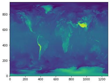
plt.figure(figsize=(6, 6))
plt.imshow(diff.to_array()[0,...,0], origin='lower')
CPU times: user 234 ms, sys: 27.6 ms, total: 261 ms
Wall time: 6.04 s
In terms of code, compared with the local version above, this has only added the use of with blocks to label data and manage execution, and executes some 100 times faster.
This is a best case, because in the demonstrator the files are actually hosted on the worker machines, so the speed difference between reading the files locally and reading them over NFS is maximized. Perhaps more persuasive is the measured volume of network traffic.
| Method | Time Taken | Measured Network Traffic |
|---|---|---|
| Calculation over NFS | > 14 minutes | 2.8 GiB |
| Distributed Calculation | ~ 10 seconds | 8 MiB |
Apart from some control and status messages, only the data required to paint the picture is sent over the network to this computer.
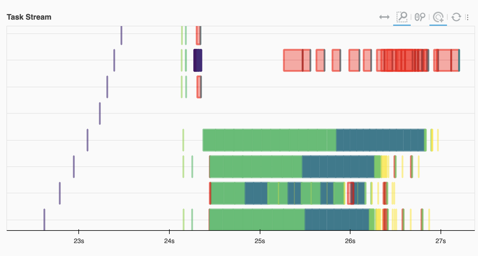
Looking at the task stream we see the ECMWF workers (on the bottom) doing the bulk of the reading and computation, with the red transfer tasks joining this with data on EUMETSAT.
Image(filename="images/task-graph.png")
Catalogs
We can simplify this code even more. Because the data-loading tasks are labelled with their resource pool, this can be opaque to the scientist. So we can write
def load_from_catalog(path):
    with pool(path.split('/')[2]):
        return xarray.open_dataset(path).chunk('auto')
allowing us to ignore where the data came from
predictions = load_from_catalog('/data/ecmwf/000490262cdd067721a34112963bcaa2b44860ab.nc')
observations = load_from_catalog('/data/eumetsat/ad-hoc/observations.nc')

averages = predictions.mean('realization')
diff = averages.isel(height=10) - observations

with propagate_pools():
    show_all_workers()
    diff.compute()
Of course the cluster would have to be provisioned with compute resources in the appropriate data centres, although with some work this could be made dynamic as part of the catalog code.
More Information
This notebook, and the code behind it, are published in a GitHub repository.
For details of the prototype implementation, and ideas for enhancements, see dask-multi-cloud-details.ipynb.
Acknowledgements
Thank you to Armagan Karatosun (EUMETSAT) and Vasileios Baousis (ECMWF) for their help and support with the infrastructure to support this proof of concept. Gabe Joseph (Coiled) wrote the clever pool context managers, and Jacob Tomlinson (NVIDIA) reviewed this document.
Crown Copyright 2022
blog comments powered by Disqus