Dask and the __array_function__ protocol Advances on NEP-18
By Peter Andreas Entschev
Summary
Dask is versatile for analytics parallelism, but there is still one issue to
leverage it to a broader spectrum: allowing it to transparently work with
NumPy-like libraries. We have previously discussed
how to work with
GPU Dask Arrays,
but limited to the scope of the array’s member methods sharing a NumPy-like
interface, for example the .sum() method, thus, calling general functionality
from NumPy’s library wasn’t still possible. NumPy recently addressed this issue
in NEP-18
with the introduction of the __array_function__ protocol. In short, the
protocol allows a NumPy function call to dispatch the appropriate NumPy-like
library implementation, depending on the array type given as input, thus
allowing Dask to remain agnostic of such libraries, internally calling just the
NumPy function, which automatically handles dispatching of the appropriate
library implementation, for example,
CuPy or Sparse.
To understand what’s the end goal of this change, consider the following example:
import numpy as np
import dask.array as da

x = np.random.random((5000, 1000))

d = da.from_array(x, chunks=(1000, 1000))

u, s, v = np.linalg.svd(d)
Now consider we want to speedup the SVD computation of a Dask array and offload
that work to a CUDA-capable GPU, we ultimately want to simply replace the NumPy
array x by a CuPy array and let NumPy do its magic via
__array_function__ protocol and dispatch the appropriate CuPy linear algebra
operations under the hood:
import numpy as np
import cupy
import dask.array as da

x = cupy.random.random((5000, 1000))

d = da.from_array(x, chunks=(1000, 1000))

u, s, v = np.linalg.svd(d)
We could do the same for a Sparse array, or any other NumPy-like array that
supports the __array_function__ protocol and the computation that we are
trying to perform. In the next section, we will take a look at potential
performance benefits that the protocol helps leveraging.
Note that the features described in this post are still experimental, some
still under development and review. For a more detailed discussion on the
actual progress of __array_function__, please refer to the Issues section.
Performance
Before going any further, assume the following hardware is utilized for all performance results described in this entire post:
- CPU: 6-core (12-threads) Intel Core i7-7800X @ 3.50GHz
- Main memory: 16 GB
- GPU: NVIDIA Quadro GV100
- OpenBLAS 0.2.18
- cuBLAS 9.2.174
- cuSOLVER 9.2.148
Let’s now check an example to see potential performance benefits of the
__array_function__ protocol with Dask when using CuPy as a backend. Let’s
start by creating all the arrays that we will use for computing an SVD later.
Please note that my focus here is how Dask can leverage compute performance,
therefore I’m ignoring in this example the time spent on creating or copying
the arrays between CPU and GPU.
import numpy as np
import cupy
import dask.array as da

x = np.random.random((10000, 1000))
y = cupy.array(x)

dx = da.from_array(x, chunks=(5000, 1000))
dy = da.from_array(y, chunks=(5000, 1000), asarray=False)
Seen above we have four arrays:
x: a NumPy array in main memory;y: a CuPy array in GPU memory;dx: a NumPy array wrapped in a Dask array;dy: a copy of a CuPy array wrapped in a Dask array; wrapping a CuPy array in a Dask array as a view (asarray=True) is not supported yet.
Compute SVD on a NumPy array
We can then start by computing the SVD of x using NumPy, thus, it’s
processed on CPU in a single thread:
u, s, v = np.linalg.svd(x)
The timing information I obtained after that looks like the following:
CPU times: user 3min 10s, sys: 347 ms, total: 3min 11s
Wall time: 3min 11s
Over 3 minutes seems a bit too slow, so now the question is: Can we do better, and more importantly, without having to change our entire code?
The answer to this question is: Yes, we can.
Let’s look now at other results.
Compute SVD on the NumPy array wrapped in Dask array
First, of all, this is what you had to do before the introduction of the
__array_function__ protocol:
u, s, v = da.linalg.svd(dx)
u, s, v = dask.compute(u, s, v)
The code above might have been very prohibitive for several projects, since one
needs to call the proper library dispatcher in addition to passing the correct
array. In other words, one would need to find all NumPy calls in the code and
replace those by the correct library’s function call, depending on the input
array type. After __array_function__, the same NumPy function can be
called, using the Dask array dx as input:
u, s, v = np.linalg.svd(dx)
u, s, v = dask.compute(u, s, v)
Note: Dask defers computation of results until its consumption, therefore we
need to call the dask.compute() function on result arrays to actually compute
them.
Let’s now take a look at the timing information:
CPU times: user 1min 23s, sys: 460 ms, total: 1min 23s
Wall time: 1min 13s
Now, without changing any code, besides the wrapping of the NumPy array as a Dask array, we can see a speedup of 2x. Not too bad. But let’s go back to our previous question: Can we do better?
Compute SVD on the CuPy array
We can do the same as for the Dask array now and simply call NumPy’s SVD
function on the CuPy array y:
u, s, v = np.linalg.svd(y)
The timing information we get now is the following:
CPU times: user 17.3 s, sys: 1.81 s, total: 19.1 s
Wall time: 19.1 s
We now see a 4-5x speedup with no change in internal calls whatsoever! This is
exactly the sort of benefit that we expect to leverage with the
__array_function__ protocol, speeding up existing code, for free!
Let’s go back to our original question one last time: Can we do better?
Compute SVD on the CuPy array wrapped in Dask array
We can now take advantage of the benefits of Dask data chunk splitting and the CuPy GPU implementation, in an attempt to keep our GPU busy as much as possible, this remains as simple as:
u, s, v = np.linalg.svd(dy)
u, s, v = dask.compute(u, s, v)
For which we get the following timing:
CPU times: user 8.97 s, sys: 653 ms, total: 9.62 s
Wall time: 9.45 s
Giving us another 2x speedup over the single-threaded CuPy SVD computing.
To conclude, we started from over 3 minutes and are now down to under 10 seconds by simply dispatching the work on a different array.
Application
We will now talk a bit about potential applications of the
__array_function__ protocol. For this, we will discuss the
Dask-GLM library, used for fitting
Generalized Linear Models on large datasets. It’s built on top of Dask and
offers an API compatible with scikit-learn.
Before the introduction of the __array_function__ protocol, we would need
to rewrite most of its internal implementation for each and every NumPy-like
library that we wished to use as a backend, therefore, we would need a
specialization of the implementation for Dask, another for CuPy and yet
another for Sparse. Now, thanks to all the functionality that these libraries
share through compatible interface, we don’t have to change the implementation
at all, we simply pass a different array type as input, as simple as that.
Example with scikit-learn
To demonstrate the ability we acquired, let’s consider the following scikit-learn example (based on the original example here):
import numpy as np
import matplotlib.pyplot as plt
from sklearn.linear_model import LinearRegression

N = 1000

# x from 0 to N
x = N * np.random.random((40000, 1))

# y = a*x + b with noise
y = 0.5 * x + 1.0 + np.random.normal(size=x.shape)

# create a linear regression model
est = LinearRegression()
We can then fit the model,
est.fit(x, y)
and obtain its time measurements:
CPU times: user 3.4 ms, sys: 0 ns, total: 3.4 ms
Wall time: 2.3 ms
We can then use it for prediction on some test data,
# predict y from the data
x_new = np.linspace(0, N, 100)
y_new = est.predict(x_new[:, np.newaxis])
And also check its time measurements:
CPU times: user 1.16 ms, sys: 680 µs, total: 1.84 ms
Wall time: 1.58 ms
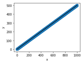
And finally plot the results:
# plot the results
plt.figure(figsize=(4, 3))
ax = plt.axes()
ax.scatter(x, y, linewidth=3)
ax.plot(x_new, y_new, color='black')

ax.set_facecolor((1.0, 1.0, 0.42))

ax.set_xlabel('x')
ax.set_ylabel('y')

ax.axis('tight')

plt.show()
Example with Dask-GLM
The only thing we have to change from the code before is the first block, where we import libraries and create arrays:
import numpy as np
from dask_glm.estimators import LinearRegression
import matplotlib.pyplot as plt

N = 1000

# x from 0 to N
x = N * np.random.random((40000, 1))

# y = a*x + b with noise
y = 0.5 * x + 1.0 + np.random.normal(size=x.shape)

# create a linear regression model
est = LinearRegression(solver='lbfgs')
The rest of the code and also the plot look alike the previous scikit-learn
example, so we’re ommitting those here for brevity. Note also that we could
have called LinearRegression() without any arguments, but for this example
we chose the
lbfgs
solver, that converges reasonably fast.
We can also have a look at the timing results for fitting, followed by those for predicting with Dask-GLM:
# Fitting
CPU times: user 9.66 ms, sys: 116 µs, total: 9.78 ms
Wall time: 8.94 ms

# Predicting
CPU times: user 130 µs, sys: 327 µs, total: 457 µs
Wall time: 1.06 ms
If instead we want to use CuPy to compute, we have to change only 3 lines,
importing cupy instead of numpy, and the two lines where we create the
random arrays, replacing them to cupy.random insted of np.random. The
block should then look like this:
import cupy
from dask_glm.estimators import LinearRegression
import matplotlib.pyplot as plt

N = 1000

# x from 0 to N
x = N * cupy.random.random((40000, 1))

# y = a*x + b with noise
y = 0.5 * x + 1.0 + cupy.random.normal(size=x.shape)

# create a linear regression model
est = LinearRegression(solver='lbfgs')
And the timing results we obtain in this scenario are:
# Fitting
CPU times: user 151 ms, sys: 40.7 ms, total: 191 ms
Wall time: 190 ms

# Predicting
CPU times: user 1.91 ms, sys: 778 µs, total: 2.69 ms
Wall time: 1.37 ms
For the simple example chosen for this post, scikit-learn outperforms Dask-GLM using both NumPy and CuPy arrays. There may exist several reasons that contribute to this, and while we didn’t dive deep into understanding the exact reasons and their extent, we could cite some likely possibilities:
- scikit-learn may be using solvers that converge faster;
- Dask-GLM is entirely built on top of Dask, while scikit-learn may be heavily optimized internally;
- Too many synchronization steps and data transfer could occur for small datasets with CuPy.
Performance for different Dask-GLM solvers
To verify how Dask-GLM with NumPy arrays would compare with CuPy arrays, we also did some logistic regression benchmarking of Dask-GLM solvers. The results below were obtained from a training dataset with 102, 103, …, 106 features of 100 dimensions, and matching number of test features.
Note: we are intentionally omitting results for Dask arrays, as we have identified a potential bug that causes Dask arrays not to converge.
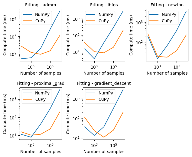
From the results observed in the graphs above we can see that CuPy can be one order of magnitude faster than NumPy for fitting with any of the Dask-GLM solvers. Please note also that both axis are given in logarithmic scale for easier visualization.
Another interesting effect that can be seen is how converging may take longer for small number of samples. However, as we would normally hope for, compute time required to converge scales linearly to the number of samples.
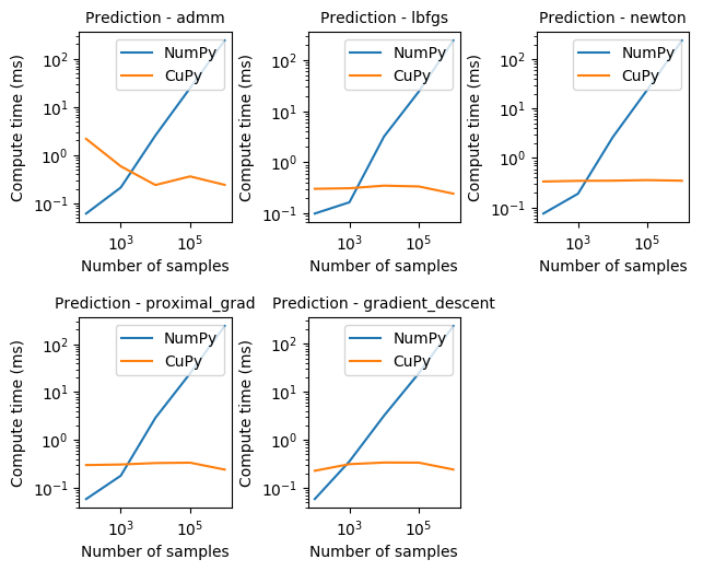
Prediction with CuPy, as seen above, can be proportionally much faster than NumPy, staying mostly constant for all solvers, and around 3-4 orders of magnitude faster.
Issues
In this section we describe the work that has been done and is still ongoing since February, 2019, towards enabling the features described in previous sections. If you are not interested in all the details, feel free to completely skip this.
Fixed Issues
Since early February, 2019, substantial progress has been made towards deeper
support of the __array_function__ protocol in the different projects,
this trend is still going on and will continue in March. Below we see a list
of issues that have been fixed or are in the process of review:
__array_function__protocol dependencies fixed in CuPy PR #2029;- Dask issues using CuPy backend with mean() and moment() Dask Issue #4481, fixed in Dask PR #4513 and Dask PR #4519;
- Replace in SciPy the aliased NumPy functions that may not be available in libraries like CuPy, fixed in SciPy PR #9888;
- Allow creation of arbitrary shaped arrays, using the input array as reference for the new array to be created, under review in NumPy PR #13043;
- Multithreading with CuPy first identified in Dask Issue #4487, CuPy Issue #2045 and CuPy Issue #1109, now under review in CuPy PR #2053;
- Calling Dask’s
flatnonzero()on CuPy array missingcupy.compress(), first identified in Dask Issue #4497, under review in Dask PR #4548, - Dask support for
__array_function__, under review in Dask PR #4567.
Known Issues
Currently, one of the biggest issues we are tackling relates to the
Dask issue #4490 we first
identified when calling Dask’s diag() on a CuPy array. This requires some
change on the Dask Array class, and subsequent changes throughout large
parts of the Dask codebase. I will not go into too much detail here, but the
way we are handling this issue is by adding a new attribute _meta to Dask
Array in replacement of the simple dtype that currently exists. This
new attribute will not only hold the dtype information, but also an empty
array of the backend type used to create the Array in the first place, thus
allowing us to internally reconstruct arrays of the backend type, without
having to know explicitly whether it’s a NumPy, CuPy, Sparse or any other
NumPy-like array. For additional details, please refer to Dask Issue
#2977.
We have identified some more issues with ongoing discussions:
- Using Sparse as a Dask backend, discussed in Dask Issue #4523;
- Calling Dask’s
fix()on CuPy array depends on__array_wrap__, discussed in Dask Issue #4496 and CuPy Issue #589; - Allow coercing of
__array_function__, discussed in NumPy Issue #12974.
Future Work
There are several possibilities for a richer experience with Dask, some of which could be very interesting in the short and mid-term are:
-
Use Dask-cuDF alongside with Dask-GLM to present interesting realistic applications of the whole ecosystem;
-
More comprehensive examples and benchmarks for Dask-GLM;
-
Support for more models in Dask-GLM;
-
A deeper look into the Dask-GLM versus scikit-learn performance;
-
Profile CuPy’s performance of matrix-matrix multiplication operations (GEMM), compare to matrix-vector multiplication operations (GEMV) for distributed Dask operation.
blog comments powered by Disqus