Dask and Scikit-Learn -- Model Parallelism Parallelizing Grid Search with Dask
By Jim Crist
This post was written by Jim Crist. The original post lives at http://jcrist.github.io/dask-sklearn-part-1.html (with better styling)
This is the first of a series of posts discussing some recent experiments combining dask and scikit-learn. A small (and extremely alpha) library has been built up from these experiments, and can be found here.
Before we start, I would like to make the following caveats:
- I am not a machine learning expert. Do not consider this a guide on how to do machine learning, the usage of scikit-learn below is probably naive.
- All of the code discussed here is in flux, and shouldn’t be considered stable or robust. That said, if you know something about machine learning and want to help out, I’d be more than happy to receive issues or pull requests :).
There are several ways of parallelizing algorithms in machine learning. Some algorithms can be made to be data-parallel (either across features or across samples). In this post we’ll look instead at model-parallelism (use same data across different models), and dive into a daskified implementation of GridSearchCV.
What is grid search?
Many machine learning algorithms have hyperparameters which can be tuned to improve the performance of the resulting estimator. A grid search is one way of optimizing these parameters — it works by doing a parameter sweep across a cartesian product of a subset of these parameters (the “grid”), and then choosing the best resulting estimator. Since this is fitting many independent estimators across the same set of data, it can be fairly easily parallelized.
Grid search with scikit-learn
In scikit-learn, a grid search is performed using the GridSearchCV class, and
can (optionally) be automatically parallelized using
joblib.
This is best illustrated with an example. First we’ll make an example dataset for doing classification against:
from sklearn.datasets import make_classification

X, y = make_classification(n_samples=10000,
                           n_features=500,
                           n_classes=2,
                           n_redundant=250,
                           random_state=42)
To solve this classification problem, we’ll create a pipeline of a PCA and a
LogisticRegression:
from sklearn import linear_model, decomposition
from sklearn.pipeline import Pipeline

logistic = linear_model.LogisticRegression()
pca = decomposition.PCA()
pipe = Pipeline(steps=[('pca', pca),
                       ('logistic', logistic)])
Both of these classes take several hyperparameters, we’ll do a grid-search across only a few of them:
#Parameters of pipelines can be set using ‘__’ separated parameter names:
grid = dict(pca__n_components=[50, 100, 250],
            logistic__C=[1e-4, 1.0, 1e4],
            logistic__penalty=['l1', 'l2'])
Finally, we can create an instance of GridSearchCV, and perform the grid
search. The parameter n_jobs=-1 tells joblib to use as many processes as I
have cores (8).
>>> from sklearn.grid_search import GridSearchCV
>>> estimator = GridSearchCV(pipe, grid, n_jobs=-1)
>>> %time estimator.fit(X, y)
CPU times: user 5.3 s, sys: 243 ms, total: 5.54 s
Wall time: 21.6 s
What happened here was:
- An estimator was created for each parameter combination and test-train set (scikit-learn’s grid search also does cross validation across 3-folds by default).
- Each estimator was fit on its corresponding set of training data
- Each estimator was then scored on its corresponding set of testing data
- The best set of parameters was chosen based on these scores
- A new estimator was then fit on all of the data, using the best parameters
The corresponding best score, parameters, and estimator can all be found as attributes on the resulting object:
>>> estimator.best_score_
0.89290000000000003

>>> estimator.best_params_
{'logistic__C': 0.0001, 'logistic__penalty': 'l2', 'pca__n_components': 50}

>>> estimator.best_estimator_
Pipeline(steps=[('pca', PCA(copy=True, n_components=50, whiten=False)), ('logistic', LogisticRegression(C=0.0001, class_weight=None, dual=False,
        fit_intercept=True, intercept_scaling=1, max_iter=100,
        multi_class='ovr', n_jobs=1, penalty='l2', random_state=None,
        solver='liblinear', tol=0.0001, verbose=0, warm_start=False))])<div class=md_output>

    {'logistic__C': 0.0001, 'logistic__penalty': 'l2', 'pca__n_components': 50}
Grid search with dask-learn
Here we’ll repeat the same fit using dask-learn. I’ve tried to match the
scikit-learn interface as much as possible, although not everything is
implemented. Here the only thing that really changes is the GridSearchCV
import. We don’t need the n_jobs keyword, as this will be parallelized across
all cores by default.
>>> from dklearn.grid_search import GridSearchCV as DaskGridSearchCV
>>> destimator = DaskGridSearchCV(pipe, grid)
>>> %time destimator.fit(X, y)

CPU times: user 16.3 s, sys: 1.89 s, total: 18.2 s
Wall time: 5.63 s
As before, the best score, parameters, and estimator can all be found as attributes on the object. Here we’ll just show that they’re equivalent:
>>> destimator.best_score_ == estimator.best_score_
True

>>> destimator.best_params_ == estimator.best_params_
True

>>> destimator.best_estimator_
Pipeline(steps=[('pca', PCA(copy=True, n_components=50, whiten=False)), ('logistic', LogisticRegression(C=0.0001, class_weight=None, dual=False,
        fit_intercept=True, intercept_scaling=1, max_iter=100,
        multi_class='ovr', n_jobs=1, penalty='l2', random_state=None,
        solver='liblinear', tol=0.0001, verbose=0, warm_start=False))])<div class=md_output>

    {'logistic__C': 0.0001, 'logistic__penalty': 'l2', 'pca__n_components': 50}
Why is the dask version faster?
If you look at the times above, you’ll note that the dask version was ~4X
faster than the scikit-learn version. This is not because we have optimized any
of the pieces of the Pipeline, or that there’s a significant amount of
overhead to joblib (on the contrary, joblib does some pretty amazing things,
and I had to construct a contrived example to beat it this badly). The reason
is simply that the dask version is doing less work.
This maybe best explained in pseudocode. The scikit-learn version of the above (in serial) looks something like (pseudocode):
for X_train, X_test, y_train, y_test in cv:
    for n in grid['pca__n_components']:
        for C in grid['logistic__C']:
            for penalty in grid['logistic__penalty']:
                # Create and fit a PCA on the input data
                pca = PCA(n_components=n).fit(X_train, y_train)
                # Transform both the train and test data
                X_train2 = pca.transform(X_train)
                X_test2 = pca.transform(X_test)
                # Create and fit a LogisticRegression on the transformed data
                logistic = LogisticRegression(C=C, penalty=penalty)
                logistic.fit(X_train2, y_train)
                # Score the total pipeline
                score = logistic.score(X_test2, y_test)
                # Save the score and parameters
                scores_and_params.append((score, n, C))

# Find the best set of parameters (for some definition of best)
find_best_parameters(scores)
This is looping through a cartesian product of the cross-validation sets and all the parameter combinations, and then creating and fitting a new estimator for each combination. While embarassingly parallel, this can also result in repeated work, as earlier stages in the pipeline are refit multiple times on the same parameter + data combinations.
In contrast, the dask version hashes all inputs (forming a sort of Merkle DAG), resulting in the intermediate results being shared. Keeping with the pseudocode above, the dask version might look like:
for X_train, X_test, y_train, y_test in cv:
    for n in grid['pca__n_components']:
        # Create and fit a PCA on the input data
        pca = PCA(n_components=n).fit(X_train, y_train)
        # Transform both the train and test data
        X_train2 = pca.transform(X_train)
        X_test2 = pca.transform(X_test)
        for C in grid['logistic__C']:
            for penalty in grid['logistic__penalty']:
                # Create and fit a LogisticRegression on the transformed data
                logistic = LogisticRegression(C=C, penalty=penalty)
                logistic.fit(X_train2, y_train)
                # Score the total pipeline
                score = logistic.score(X_test2, y_test)
                # Save the score and parameters
                scores_and_params.append((score, n, C, penalty))

# Find the best set of parameters (for some definition of best)
find_best_parameters(scores)
This can still be parallelized, but in a less straightforward manner - the graph is a bit more complicated than just a simple map-reduce pattern. Thankfully the dask schedulers are well equipped to handle arbitrary graph topologies. Below is a GIF showing how the dask scheduler (the threaded scheduler specifically) executed the grid search performed above. Each rectangle represents data, and each circle represents a task. Each is categorized by color:
-
Red means actively taking up resources. These are tasks executing in a thread, or intermediate results occupying memory
-
Blue means finished or released. These are already finished tasks, or data that’s been released from memory because it’s no longer needed
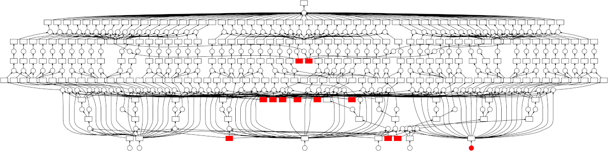
Looking at the trace, a few things stand out:
-
We do a good job sharing intermediates. Each step in a pipeline is only fit once given the same parameters/data, resulting in some intermediates having many dependent tasks.
-
The scheduler does a decent job of quickly finishing up tasks required to release data. This doesn’t matter as much here (none of the intermediates take up much memory), but for other workloads this is very useful. See Matt Rocklin’s excellent blogpost here for more discussion on this.
Distributed grid search using dask-learn
The schedulers used in dask are configurable. The default (used above) is the threaded scheduler, but we can just as easily swap it out for the distributed scheduler. Here I’ve just spun up two local workers to demonstrate, but this works equally well across multiple machines.
>>> from distributed import Executor

>>> # Create an Executor, and set it as the default scheduler
>>> exc = Executor('10.0.0.3:8786', set_as_default=True)
>>> exc
<Executor: scheduler="10.0.0.3:8786" processes=2 cores=8>

>>> %time destimator.fit(X, y)
CPU times: user 1.69 s, sys: 433 ms, total: 2.12 s
Wall time: 7.66 s

>>> %time destimator.fit(X, y)
CPU times: user 1.69 s, sys: 433 ms, total: 2.12 s
Wall time: 7.66 s

>>> (destimator.best_score_ == estimator.best_score_ and
...  destimator.best_params_ == estimator.best_params_)
True
Note that this is slightly slower than the threaded execution, so it doesn’t make sense for this workload, but for others it might.
What worked well
-
The code for doing this is quite short. There’s also an implementation of
RandomizedSearchCV, which is only a few extra lines (hooray for good class hierarchies!). Instead of working with dask graphs directly, both implementations use dask.delayed wherever possible, which also makes the code easy to read. -
Due to the internal hashing used in dask (which is extensible!), duplicate computations are avoided.
-
Since the graphs are separated from the scheduler, this works both locally and distributed with only a few extra lines.
Caveats and what could be better
-
The scikit-learn api makes use of mutation (
est.fit(X, y)mutatesest), while dask collections are mostly immutable. After playing around with a few different ideas, I settled on dask-learn estimators being immutable (except for grid-search, more on this in a bit). This made the code easier to reason about, but does mean that you need to doest = est.fit(X, y)when working with dask-learn estimators. -
GridSearchCVposed a different problem. Due to therefitkeyword, the implementation can’t be done in a single pass over the data. This means that we can’t build a single graph describing both the grid search and the refit, which prevents it from being done lazily. I debated removing this keyword, but decided in the end to makefitexecute immediately. This means that there’s a bit of a disconnect betweenGridSearchCVand the other classes in the library, which I don’t like. On the other hand, it does mean that this version ofGridSearchCVcould be a drop-in for the sckit-learn one. -
The approach presented here is nice, but is really only beneficial when there’s duplicate work to be avoided, and that duplicate work is expensive. Repeating the above with only a single estimator (instead of a pipeline) results in identical (or slightly worse) performance than joblib. Similarly, if the repeated steps are cheap the difference in performance is much smaller (try the above using SelectKBest instead of
PCA). -
The ability to swap easily from local to distributed execution is nice, but distributed also contains a joblib frontend that can do this just as easily.
Help
I am not a machine learning expert. Is any of this useful? Do you have suggestions for improvements (or better yet PRs for improvements :))? Please feel free to reach out in the comments below, or on github.
This work is supported by Continuum Analytics and the XDATA program as part of the Blaze Project.
blog comments powered by Disqus