Towards Out-of-core DataFrames
This work is supported by Continuum Analytics and the XDATA Program as part of the Blaze Project
This post primarily targets developers. It is on experimental code that is not ready for users.
tl;dr Can we build dask.frame? One approach involves indexes and a lot
of shuffling.
Dask arrays work
Over the last two months we’ve watched the creation of
dask, a task scheduling specification, and
dask.array a project to
implement the out-of-core nd-arrays using blocked algorithms.
(blogposts:
1,
2,
3,
4,
5,
6).
This worked pretty well. Dask.array is available on the main conda channel and on PyPI
and, for the most part, is a pleasant drop-in replacement for a subset of NumPy
operations. I’m really happy with it.
conda install dask
or
pip install dask
There is still work to do, in particular I’d like to interact with people who
have real-world problems, but for the most part dask.array feels ready.
On to dask frames
Can we do for Pandas what we’ve just done for NumPy?
Question: Can we represent a large DataFrame as a sequence of in-memory DataFrames and perform most Pandas operations using task scheduling?
Answer: I don’t know. Lets try.
Naive Approach
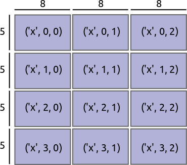
If represent a dask.array as an N-d grid of NumPy ndarrays, then maybe we should represent a dask.frame as a 1-d grid of Pandas DataFrames; they’re kind of like arrays.
| dask.array | Naive dask.frame | |
 |
 |
This approach supports the following operations:
- Elementwise operations
df.a + df.b - Row-wise filtering
df[df.a > 0] - Reductions
df.a.mean() - Some split-apply-combine operations that combine with a standard reduction
like
df.groupby('a').b.mean(). Essentially anything you can do withdf.groupby(...).agg(...)
The reductions and split-apply-combine operations require some cleverness. This is how Blaze works now and how it does the does out-of-core operations in these notebooks: Blaze and CSVs, Blaze and Binary Storage.
However this approach does not support the following operations:
- Joins
- Split-apply-combine with more complex
transformorapplycombine steps - Sliding window or resampling operations
- Anything involving multiple datasets
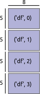
Partition on the Index values
Instead of partitioning based on the size of blocks we instead partition on value ranges of the index.
| Partition on block size | Partition on index value | |
|
 |
This opens up a few more operations
- Joins are possible when both tables share the same index. Because we have information about index values we we know which blocks from one side need to communicate to which blocks from the other.
- Split-apply-combine with transform/apply steps are possible when the grouper
is the index. In this case we’re guaranteed that each group is in the same
block. This opens up general
df.gropuby(...).apply(...) - Rolling or resampling operations are easy on the index if we share a small
amount of information between blocks as we do in
dask.arrayfor ghosting operations.
We note the following theme:
Complex operations are easy if the logic aligns with the index
And so a recipe for many complex operations becomes:
- Re-index your data along the proper column
- Perform easy computation
Re-indexing out-of-core data
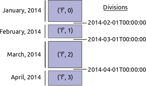
To be explicit imagine we have a large time-series of transactions indexed by time and partitioned by day. The data for every day is in a separate DataFrame.
Block 1
-------
                     credit    name
time
2014-01-01 00:00:00     100     Bob
2014-01-01 01:00:00     200   Edith
2014-01-01 02:00:00    -300   Alice
2014-01-01 03:00:00     400     Bob
2014-01-01 04:00:00    -500  Dennis
...

Block 2
-------
                     credit    name
time
2014-01-02 00:00:00     300    Andy
2014-01-02 01:00:00     200   Edith
...
We want to reindex this data and shuffle all of the entries so that now we partiion on the name of the person. Perhaps all of the A’s are in one block while all of the B’s are in another.
Block 1
-------
                       time  credit
name
Alice   2014-04-30 00:00:00     400
Alice   2014-01-01 00:00:00     100
Andy    2014-11-12 00:00:00    -200
Andy    2014-01-18 00:00:00     400
Andy    2014-02-01 00:00:00    -800
...

Block 2
-------
                       time  credit
name
Bob     2014-02-11 00:00:00     300
Bob     2014-01-05 00:00:00     100
...
Re-indexing and shuffling large data is difficult and expensive. We need to find good values on which to partition our data so that we get regularly sized blocks that fit nicely into memory. We also need to shuffle entries from all of the original blocks to all of the new ones. In principle every old block has something to contribute to every new one.
We can’t just call DataFrame.sort because the entire data might not fit in
memory and most of our sorting algorithms assume random access.
We do this in two steps
- Find good division values to partition our data. These should partition the data into blocks of roughly equal size.
- Shuffle our old blocks into new blocks along the new partitions found in step one.
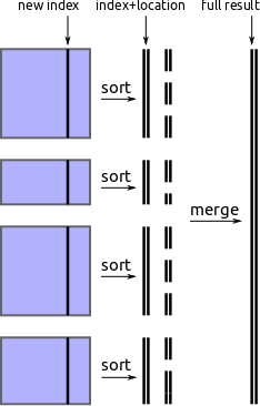
Find divisions by external sorting
One approach to find new partition values is to pull out the new index from each block, perform an out-of-core sort, and then take regularly spaced values from that array.
-
Pull out new index column from each block
indexes = [block['new-column-index'] for block in blocks] -
Perform out-of-core sort on that column
sorted_index = fancy_out_of_core_sort(indexes) -
Take values at regularly spaced intervals, e.g.
partition_values = sorted_index[::1000000]
We implement this using parallel in-block sorts, followed by a streaming merge
process using the heapq module. It works but is slow.
Possible Improvements
This could be accelerated through one of the following options:
- A streaming numeric solution that works directly on iterators of NumPy
arrays (
numtoolzanyone?) - Not sorting at all. We only actually need approximate regularly spaced quantiles. A brief literature search hints that there might be some good solutions.
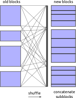
Shuffle
Now that we know the values on which we want to partition we ask each block to
shard itself into appropriate pieces and shove all of those pieces into a
spill-to-disk dictionary. Another process then picks up these pieces and calls
pd.concat to merge them in to the new blocks.
For the out-of-core dict we’re currently using Chest. Turns out that serializing DataFrames and writing them to disk can be tricky. There are several good methods with about an order of magnitude performance difference between them.
This works but my implementation is slow
Here is an example with snippet of the NYCTaxi data (this is small)
In [1]: import dask.frame as dfr

In [2]: d = dfr.read_csv('/home/mrocklin/data/trip-small.csv', chunksize=10000)

In [3]: d.head(3)   # This is fast
Out[3]:
                          medallion                      hack_license  \
0  89D227B655E5C82AECF13C3F540D4CF4  BA96DE419E711691B9445D6A6307C170
1  0BD7C8F5BA12B88E0B67BED28BEA73D8  9FD8F69F0804BDB5549F40E9DA1BE472
2  0BD7C8F5BA12B88E0B67BED28BEA73D8  9FD8F69F0804BDB5549F40E9DA1BE472

  vendor_id  rate_code store_and_fwd_flag      pickup_datetime  \
0       CMT          1                  N  2013-01-01 15:11:48
1       CMT          1                  N  2013-01-06 00:18:35
2       CMT          1                  N  2013-01-05 18:49:41

      dropoff_datetime  passenger_count  trip_time_in_secs  trip_distance  \
0  2013-01-01 15:18:10                4                382            1.0
1  2013-01-06 00:22:54                1                259            1.5
2  2013-01-05 18:54:23                1                282            1.1

   pickup_longitude  pickup_latitude  dropoff_longitude  dropoff_latitude
0        -73.978165        40.757977         -73.989838         40.751171
1        -74.006683        40.731781         -73.994499         40.750660
2        -74.004707        40.737770         -74.009834         40.726002

In [4]: d2 = d.set_index(d.passenger_count, out_chunksize=10000)   # This takes some time

In [5]: d2.head(3)
Out[5]:
                                        medallion  \
passenger_count
0                3F3AC054811F8B1F095580C50FF16090
1                4C52E48F9E05AA1A8E2F073BB932E9AA
1                FF00E5D4B15B6E896270DDB8E0697BF7

                                     hack_license vendor_id  rate_code  \
passenger_count
0                E00BD74D8ADB81183F9F5295DC619515       VTS          5
1                307D1A2524E526EE08499973A4F832CF       VTS          1
1                0E8CCD187F56B3696422278EBB620EFA       VTS          1

                store_and_fwd_flag      pickup_datetime     dropoff_datetime  \
passenger_count
0                              NaN  2013-01-13 03:25:00  2013-01-13 03:42:00
1                              NaN  2013-01-13 16:12:00  2013-01-13 16:23:00
1                              NaN  2013-01-13 15:05:00  2013-01-13 15:15:00

                 passenger_count  trip_time_in_secs  trip_distance  \
passenger_count
0                              0               1020           5.21
1                              1                660           2.94
1                              1                600           2.18

                 pickup_longitude  pickup_latitude  dropoff_longitude  \
passenger_count
0                      -73.986900        40.743736         -74.029747
1                      -73.976753        40.790123         -73.984802
1                      -73.982719        40.767147         -73.982170

                 dropoff_latitude
passenger_count
0                       40.741348
1                       40.758518
1                       40.746170

In [6]: d2.blockdivs  # our new partition values
Out[6]: (2, 3, 6)

In [7]: d.blockdivs   # our original partition values
Out[7]: (10000, 20000, 30000, 40000, 50000, 60000, 70000, 80000, 90000)
Some Problems
-
First, we have to evaluate the dask as we go. Every
set_indexoperation (and hence many groupbys and joins) forces an evaluation. We can no longer, as in the dask.array case, endlessly compound high-level operations to form more and more complex graphs and then only evaluate at the end. We need to evaluate as we go. -
Sorting/shuffling is slow. This is for a few reasons including the serialization of DataFrames and sorting being hard.
-
How feasible is it to frequently re-index a large amount of data? When do we reach the stage of “just use a database”?
-
Pandas doesn’t yet release the GIL, so this is all single-core. See post on PyData and the GIL.
-
My current solution lacks basic functionality. I’ve skipped the easy things to first ensure sure that the hard stuff is doable.
Help
I know less about tables than about arrays. I’m ignorant of the literature and common solutions in this field. If anything here looks suspicious then please speak up. I could really use your help.
Additionally the Pandas API is much more complex than NumPy’s. If any experienced devs out there feel like jumping in and implementing fairly straightforward Pandas features in a blocked way I’d be obliged.
blog comments powered by Disqus