Towards Out-of-core ND-Arrays -- Slicing and Stacking
This work is supported by Continuum Analytics and the XDATA Program as part of the Blaze Project
tl;dr Dask.arrays can slice and stack. This is useful for weather data.
Introduction
This is the sixth in a sequence of posts constructing an out-of-core nd-array using NumPy, and dask. You can view these posts here:
- Simple task scheduling,
- Frontend usability
- A multi-threaded scheduler
- Matrix Multiply Benchmark
- Spilling to disk
Now we talk about slicing and stacking. We use meteorological data as an example use case.
Slicing
Dask.array now supports most of the NumPy slicing syntax. In particular it supports the following:
- Slicing by integers and slices
x[0, :5] - Slicing by a
list/np.ndarrayof integersx[[1, 2, 4]] - Slicing by a
list/np.ndarrayof booleansx[[False, True, True, False, True]]
It does not currently support the following:
- Slicing one
dask.arraywith anotherx[x > 0] - Slicing with lists in multiple axes
x[[1, 2, 3], [3, 2, 1]]
Stack and Concatenate
We often store large arrays on disk in many different files. We
want to stack or concatenate these arrays together into one logical array.
Dask solves this problem with the stack and concatenate functions, which
stitch many arrays together into a single array, either creating a new
dimension with stack or along an existing dimension with concatenate.
Stack
We stack many existing dask arrays into a new array, creating a new dimension as we go.
>>> import dask.array as da
>>> arrays = [from_array(np.ones((4, 4)), blockshape=(2, 2))
...            for i in range(3)]  # A small stack of dask arrays

>>> da.stack(arrays, axis=0).shape
(3, 4, 4)

>>> da.stack(arrays, axis=1).shape
(4, 3, 4)

>>> da.stack(arrays, axis=2).shape
(4, 4, 3)
This creates a new dimension with length equal to the number of slices
Concatenate
We concatenate existing arrays into a new array, extending them along an existing dimension
>>> import dask.array as da
>>> arrays = [from_array(np.ones((4, 4)), blockshape=(2, 2))
...            for i in range(3)]  # small stack of dask arrays

>>> da.concatenate(arrays, axis=0).shape
(12, 4)

>>> da.concatenate(arrays, axis=1).shape
(4, 12)
Case Study with Meteorological Data
To test this new functionality we download meteorological data from the European Centre for Medium-Range Weather Forecasts. In particular we have the temperature for the Earth every six hours for all of 2014 with spatial resolution of a quarter degree. We download this data using this script (please don’t hammer their servers unnecessarily) (Thanks due to Stephan Hoyer for pointing me to this dataset).
As a result, I now have a bunch of netCDF files!
$ ls
2014-01-01.nc3  2014-03-18.nc3  2014-06-02.nc3  2014-08-17.nc3  2014-11-01.nc3
2014-01-02.nc3  2014-03-19.nc3  2014-06-03.nc3  2014-08-18.nc3  2014-11-02.nc3
2014-01-03.nc3  2014-03-20.nc3  2014-06-04.nc3  2014-08-19.nc3  2014-11-03.nc3
2014-01-04.nc3  2014-03-21.nc3  2014-06-05.nc3  2014-08-20.nc3  2014-11-04.nc3
...             ...             ...             ...             ...
>>> import netCDF4
>>> t = netCDF4.Dataset('2014-01-01.nc3').variables['t2m']
>>> t.shape
(4, 721, 1440)
The shape corresponds to four measurements per day (24h / 6h), 720 measurements North/South (180 / 0.25) and 1440 measurements East/West (360/0.25). There are 365 files.
Great! We collect these under one logical dask array, concatenating along the time axis.
>>> from glob import glob
>>> filenames = sorted(glob('2014-*.nc3'))
>>> temps = [netCDF4.Dataset(fn).variables['t2m'] for fn in filenames]

>>> import dask.array as da
>>> arrays = [da.from_array(t, blockshape=(4, 200, 200)) for t in temps]
>>> x = da.concatenate(arrays, axis=0)

>>> x.shape
(1464, 721, 1440)
Now we can play with x as though it were a NumPy array.
avg = x.mean(axis=0)
diff = x[1000] - avg
If we want to actually compute these results we have a few options
>>> diff.compute()  # compute result, return as array, float, int, whatever is appropriate
>>> np.array(diff)  # compute result and turn into `np.ndarray`
>>> diff.store(anything_that_supports_setitem)  # For out-of-core storage
Alternatively, because many scientific Python libraries call np.array on
inputs, we can just feed our da.Array objects directly in to matplotlib
(hooray for the __array__ protocol!):
>>> from matplotlib import imshow
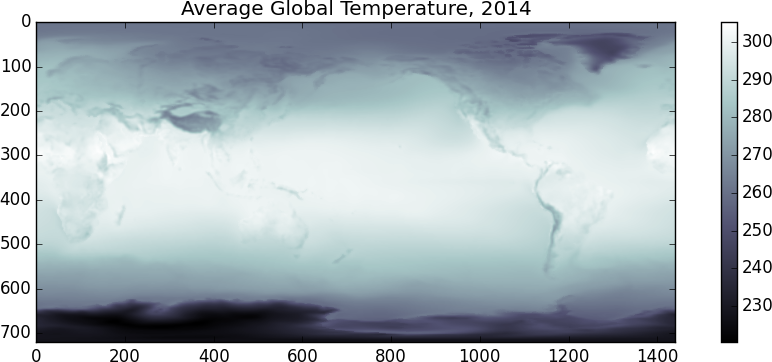
>>> imshow(x.mean(axis=0), cmap='bone')
>>> imshow(x[1000] - x.mean(axis=0), cmap='RdBu_r')
 |
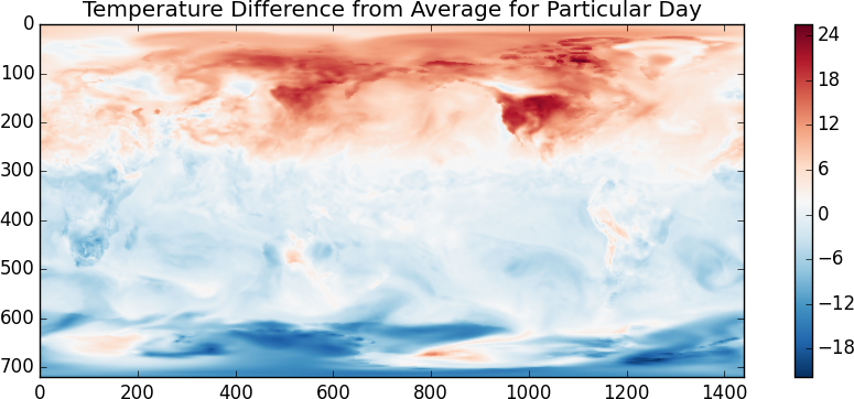 |
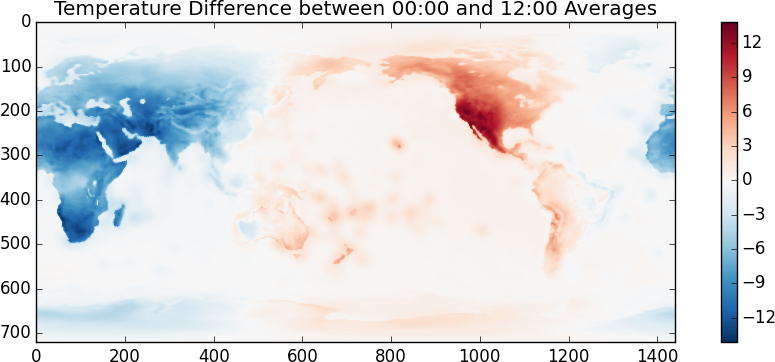
I suspect that the temperature scale is in Kelvin. It looks like the random day is taken during Northern Summer. Another fun one, lets look at the difference between the temperatures at 00:00 and at 12:00
>>> imshow(x[::4].mean(axis=0) - x[2::4].mean(axis=0), cmap='RdBu_r')
Even though this looks and feels like NumPy we’re actually operating off of disk using blocked algorithms. We execute these operations using only a small amount of memory. If these operations were computationally intense (they aren’t) then we also would also benefit from multiple cores.
What just happened
To be totally clear the following steps just occurred:
- Open up a bunch of netCDF files and located a temperature variable within each file. This is cheap.
- For each of those temperature variables create a
da.Arrayobject, specifying how we want to block up that variable. This is also cheap. - Make a new
da.Arrayby concatenating all of ourda.Arrays for each day. This, like the other steps, is just book-keeping. We haven’t loaded data or computed anything yet. - Write numpy-style code
x[::2].mean(axis=0) - x[2::2].mean(axis=0). This creates yet anotherda.Arraywith a more complex task graph. It takes a few hundred milliseconds to create this dictionary. - Call
imshowon ourda.Arrayobject imshowcallsnp.arrayon its input, this starts the multi-core task scheduler- A flurry of chunks fly out of all the netCDF files. These chunks meet
various NumPy functions and create new chunks. Well organized magic occurs
and an
np.ndarrayemerges. - Matplotlib makes a pretty graph
Problems that Popped Up
The threaded scheduler is introducing significant overhead in its planning. For this workflow the single-threaded naive scheduler is actually significantly faster. We’ll have to find better solutions to reduce scheduling overhead.
Conclusion
I hope that this shows off how dask.array can be useful when dealing with
collections of on-disk arrays. As always I’m very happy to hear how we can
make this project more useful for your work. If you have large n-dimensional
datasets I’d love to hear about what you do and how dask.array can help. I
can be reached either in the comments below or at [email protected].
Acknowledgements
First, other projects can already do this. In particular if this seemed useful
for your work then you should probably also know about
Biggus,
produced by the UK Met office, which has been around for much longer than
dask.array and is used in production.
Second, this post shows off work from the following people:
- Erik Welch (Continuum) wrote optimization passes to clean up dask graphs before execution.
- Wesley Emeneker (Continuum) wrote a good deal of the slicing code
- Stephan Hoyer (Climate Corp)
talked me through the application and pointed me to the data. If you’d
like to see dask integrated with
xraythen you should definitely bug Stephan :)
blog comments powered by Disqus