Skeleton analysis
By Genevieve Buckley
Executive Summary
In this blogpost, we show how to modify a skeleton network analysis with Dask to work with constrained RAM (eg: on your laptop). This makes it more accessible: it can run on a small laptop, instead of requiring access to a supercomputing cluster. Example code is also provided here.
Contents
- Skeleton structures are everywhere
- The scientific problem
- The compute problem
- Our approach
- Results
- Limitations
- Problems encountered
- How we solved them
- What’s next
- How you can help
Skeleton structures are everywhere
Lots of biological structures have a skeleton or network-like shape. We see these in all kinds of places, including:
- blood vessel branching
- the branching of airways
- neuron networks in the brain
- the root structure of plants
- the capillaries in leaves
- … and many more
Analysing the structure of these skeletons can give us important information about the biology of that system.
The scientific problem
For this bogpost, we will look at the blood vessels inside of a lung. This data was shared with us by Marcus Kitchen, Andrew Stainsby, and their team of collaborators.
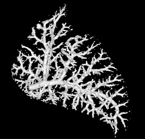
This research group focusses on lung development. We want to compare the blood vessels in a healthy lung, against a lung from a hernia model. In the hernia model the lung is underdeveloped, squashed, and smaller.
The compute problem
These image volumes have a shape of roughtly 1000x1000x1000 pixels. That doesn’t seem huge but given the high RAM consumption involved in processing the analysis, it crashes when running on a laptop.
If you’re running out of RAM, there are two possible appoaches:
-
Get more RAM. Run things on a bigger computer, or move things to a supercomputing cluster. This has the advantage that you don’t need to rewrite your code, but it does require access to more powerful computer hardware.
-
Manage the RAM you’ve got. Dask is good for this. If we use Dask, and some reasonable chunking of our arrays, we can manage things so that we never hit the RAM ceiling and crash. This has the advantage that you don’t need to buy more computer hardware, but it will require re-writing some code.
Our approach
We took the second approach, using Dask so we can run our analysis on a small laptop with constrained RAM without crashing. This makes it more accessible, to more people.
All the image pre-processing steps will be done with dask-image, and the skeletonize function of scikit-image.
We use skan as the backbone of our analysis pipeline. skan is a library for skeleton image analysis. Given a skeleton image, it can describe statistics of the branches. To make it fast, the library is accelerated with numba (if you’re curious, you can hear more about that in this talk and its related notebook).
There is an example notebook containing the full details of the skeleton analysis available here. You can read on to hear just the highlights.
Results
The statistics from the blood vessel branches in the healthy and herniated lung shows clear differences between the two.
Most striking is the difference in the number of blood vessel branches. The herniated lung has less than 40% of the number of blood vessel branches in the healthy lung.
There are also quantitative differences in the sizes of the blood vessels. Here is a violin plot showing the distribution of the distances between the start and end points of each blood vessel branch. We can see that overall the blood vessel branches start and end closer together in the herniated lung. This is consistent with what we might expect, since the healthy lung is more well developed than the lung from the hernia model and the hernia has compressed that lung into a smaller overall space.
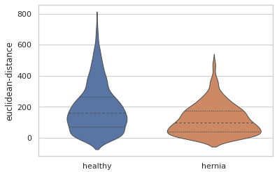
EDIT: This blogpost previously described the euclidean distance violin plot as measuring the thickness of the blood vessels. This is incorrect, and the mistake was not caught in the review process before publication. This post has been updated to correctly describe the euclidean-distance measuremet as the distance between the start and end of branches, as if you pulled a string taught between those points. An alternative measurement, branch-length describes the total branch length, including any winding twists and turns.
Limitations
We rely on one big assumption: once skeletonized the reduced non-zero pixel data will fit into memory. While this holds true for datasets of this size (the cropped rabbit lung datasets are roughly 1000 x 1000 x 1000 pixels), it may not hold true for much larger data.
Dask computation is also triggered at a few points through our prototype workflow. Ideally all computation would be delayed until the very final stage.
Problems encountered
This project was originally intended to be a quick & easy one. Famous last words!
What I wanted to do was to put the image data in a Dask array, and then use the map_overlap function to do the image filtering, thresholding, skeletonizing, and skeleton analysis. What I soon found was that although the image filtering, thresholding, and skeletonization worked well, the skeleton analysis step had some problems:
-
Dask’s map_overlap function doesn’t handle ragged or non-uniformly shaped results from different image chunks very well, and…
-
Internal function in the skan library were written in a way that was incompatible with distributed computation.
How we solved them
Problem 1: The skeletonize function from scikit-image crashes due to lack of RAM
The skeletonize function of scikit-image is very memory intensive, and was crashing on a laptop with 16GB RAM.
We solved this by:
- Putting our image data into a Dask array with dask-image
imread, - Rechunking the Dask array. We need to change the chunk shapes from 2D slices to small cuboid volumes, so the next step in the computation is efficient. We can choose the overall size of the chunks so that we can stay under the memory threshold needed for skeletonize.
- Finally, we run the
skeletonizefunction on the Dask array chunks using themap_overlapfunction. By limiting the size of the array chunks, we stay under our memory threshold!
Problem 2: Ragged or non-uniform output from Dask array chunks
The skeleton analysis functions will return results with ragged or non-uniform length for each image chunk. This is unsurpising, because different chunks will have different numbers of non-zero pixels in our skeleton shape.
When working with Dask arrays, there are two very commonly used functions: map_blocks and map_overlap. Here’s what happens when we try a function with ragged outputs with map_blocks versus map_overlap.
import dask.array as da
import numpy as np

x = da.ones((100, 10), chunks=(10, 10))

def foo(a):  # our dummy analysis function
    random_length = np.random.randint(1, 7)
    return np.arange(random_length)
With map_blocks, everything works well:
result = da.map_blocks(foo, x, drop_axis=1)
result.compute()  # this works well
But if we need some overlap for function foo to work correctly, then we run into problems:
result = da.map_overlap(foo, x, depth=1, drop_axis=1)
result.compute()  # incorrect results
Here, the first and last element of the results from foo are trimmed off before the results are concatenated, which we don’t want! Setting the keyword argument trim=False would help avoid this problem, except then we get an error:
result = da.map_overlap(foo, x, depth=1, trim=False, drop_axis=1)
result.compute()  # ValueError
Unfortunately for us, it’s really important to have a 1 pixel overlap in our array chunks, so that we can tell if a skeleton branch is ending or continuing on into the next chunk.
There’s some complexity in the way map_overlap results are concatenated back together so rather than diving into that, a more straightforward solution is to use Dask delayed instead. Chris Roat shows a nice example of how we can use Dask delayed in a list comprehension that is then concatenated with Dask (link to original discussion).
import numpy as np
import pandas as pd

import dask
import dask.array as da
import dask.dataframe as dd

x = da.ones((20, 10), chunks=(10, 10))

@dask.delayed
def foo(a):
    size = np.random.randint(1,10)  # Make each dataframe a different size
    return pd.DataFrame({'x': np.arange(size),
                         'y': np.arange(10, 10+size)})

meta = dd.utils.make_meta([('x', np.int64), ('y', np.int64)])
blocks = x.to_delayed().ravel()  # no overlap
results = [dd.from_delayed(foo(b), meta=meta) for b in blocks]
ddf = dd.concat(results)
ddf.compute()
Warning: It’s very important to pass in a meta keyword argument to the function from_delayed. Without it, things will be extremely inefficient!
If the meta keyword argument is not given, Dask will try and work out what it should be. Ordinarily that might be a good thing, but inside a list comprehension that means those tasks are computed slowly and sequentially before the main computation even begins, which is horribly inefficient. Since we know ahead of time what kinds of results we expect from our analysis function (we just don’t know the length of each set of results), we can use the utils.make_meta function to help us here.
Problem 3: Grabbing the image chunks with an overlap
Now that we’re using Dask delayed to piece together our skeleton analysis results, it’s up to us to handle the array chunks overlap ourselves.
We’ll do that by modifying Dask’s dask.array.core.slices_from_chunks function, into something that will be able to handle an overlap. Some special handling is required at the boundaries of the Dask array, so that we don’t try to slice past the edge of the array.
Here’s what that looks like (gist):
from itertools import product
from dask.array.slicing import cached_cumsum

def slices_from_chunks_overlap(chunks, array_shape, depth=1):
    cumdims = [cached_cumsum(bds, initial_zero=True) for bds in chunks]

    slices = []
    for starts, shapes in zip(cumdims, chunks):
        inner_slices = []
        for s, dim, maxshape in zip(starts, shapes, array_shape):
            slice_start = s
            slice_stop = s + dim
            if slice_start > 0:
                slice_start -= depth
            if slice_stop >= maxshape:
                slice_stop += depth
            inner_slices.append(slice(slice_start, slice_stop))
        slices.append(inner_slices)

    return list(product(*slices))
Now that we can slice an image chunk plus an extra pixel of overlap, all we need is a way to do that for all the chunks in an array. Drawing inspiration from this block iteration we make a similar iterator.
block_iter = zip(
    np.ndindex(*image.numblocks),
    map(functools.partial(operator.getitem, image),
        slices_from_chunks_overlap(image.chunks, image.shape, depth=1))
)

meta = dd.utils.make_meta([('row', np.int64), ('col', np.int64), ('data', np.float64)])
intermediate_results = [dd.from_delayed(skeleton_graph_func(block), meta=meta) for _, block in block_iter]
results = dd.concat(intermediate_results)
results = results.drop_duplicates()  # we need to drop duplicates because it counts pixels in the overlapping region twice
With these results, we’re able to create the sparse skeleton graph.
Problem 4: Summary statistics with skan
Skeleton branch statistics can be calculate with the skan summarize function. The problem here is that the function expects a Skeleton object instance, but initializing a Skeleton object calls methods that are not compatible for distributed analysis.
We’ll solve this problem by first initializing a Skeleton object instance with a tiny dummy dataset, then overwriting the attributes of the skeleton object with our real results. This is a hack, but it lets us achieve our goal: summary branch statistics for our large dataset.
First we make a Skeleton object instance with dummy data:
from skan._testdata import skeleton0

skeleton_object = Skeleton(skeleton0)  # initialize with dummy data
Then we overwrite the attributes with the previously calculated results:
skeleton_object.skeleton_image = ...
skeleton_object.graph = ...
skeleton_object.coordinates
skeleton_object.degrees = ...
skeleton_object.distances = ...
...
Then finally we can calculate the summary branch statistics:
from skan import summarize

statistics = summarize(skel_obj)
statistics.head()
| skeleton-id | node-id-src | node-id-dst | branch-distance | branch-type | mean-pixel-value | stdev-pixel-value | image-coord-src-0 | image-coord-src-1 | image-coord-src-2 | image-coord-dst-0 | image-coord-dst-1 | image-coord-dst-2 | coord-src-0 | coord-src-1 | coord-src-2 | coord-dst-0 | coord-dst-1 | coord-dst-2 | euclidean-distance | |
|---|---|---|---|---|---|---|---|---|---|---|---|---|---|---|---|---|---|---|---|---|
| 0 | 1 | 1 | 2 | 1 | 2 | 0.474584 | 0.00262514 | 22 | 400 | 595 | 22 | 400 | 596 | 22 | 400 | 595 | 22 | 400 | 596 | 1 |
| 1 | 2 | 3 | 9 | 8.19615 | 2 | 0.464662 | 0.00299629 | 37 | 400 | 622 | 43 | 392 | 590 | 37 | 400 | 622 | 43 | 392 | 590 | 33.5261 |
| 2 | 3 | 10 | 11 | 1 | 2 | 0.483393 | 0.00771038 | 49 | 391 | 589 | 50 | 391 | 589 | 49 | 391 | 589 | 50 | 391 | 589 | 1 |
| 3 | 5 | 13 | 19 | 6.82843 | 2 | 0.464325 | 0.0139064 | 52 | 389 | 588 | 55 | 385 | 588 | 52 | 389 | 588 | 55 | 385 | 588 | 5 |
| 4 | 7 | 21 | 23 | 2 | 2 | 0.45862 | 0.0104024 | 57 | 382 | 587 | 58 | 380 | 586 | 57 | 382 | 587 | 58 | 380 | 586 | 2.44949 |
statistics.describe()
| skeleton-id | node-id-src | node-id-dst | branch-distance | branch-type | mean-pixel-value | stdev-pixel-value | image-coord-src-0 | image-coord-src-1 | image-coord-src-2 | image-coord-dst-0 | image-coord-dst-1 | image-coord-dst-2 | coord-src-0 | coord-src-1 | coord-src-2 | coord-dst-0 | coord-dst-1 | coord-dst-2 | euclidean-distance | |
|---|---|---|---|---|---|---|---|---|---|---|---|---|---|---|---|---|---|---|---|---|
| count | 1095 | 1095 | 1095 | 1095 | 1095 | 1095 | 1095 | 1095 | 1095 | 1095 | 1095 | 1095 | 1095 | 1095 | 1095 | 1095 | 1095 | 1095 | 1095 | 1095 |
| mean | 2089.38 | 11520.1 | 11608.6 | 22.9079 | 2.00091 | 0.663422 | 0.0418607 | 591.939 | 430.303 | 377.409 | 594.325 | 436.596 | 373.419 | 591.939 | 430.303 | 377.409 | 594.325 | 436.596 | 373.419 | 190.13 |
| std | 636.377 | 6057.61 | 6061.18 | 24.2646 | 0.0302199 | 0.242828 | 0.0559064 | 174.04 | 194.499 | 97.0219 | 173.353 | 188.708 | 96.8276 | 174.04 | 194.499 | 97.0219 | 173.353 | 188.708 | 96.8276 | 151.171 |
| min | 1 | 1 | 2 | 1 | 2 | 0.414659 | 6.79493e-06 | 22 | 39 | 116 | 22 | 39 | 114 | 22 | 39 | 116 | 22 | 39 | 114 | 0 |
| 25% | 1586 | 6215.5 | 6429.5 | 1.73205 | 2 | 0.482 | 0.00710439 | 468.5 | 278.5 | 313 | 475 | 299.5 | 307 | 468.5 | 278.5 | 313 | 475 | 299.5 | 307 | 72.6946 |
| 50% | 2431 | 11977 | 12010 | 16.6814 | 2 | 0.552626 | 0.0189069 | 626 | 405 | 388 | 627 | 410 | 381 | 626 | 405 | 388 | 627 | 410 | 381 | 161.059 |
| 75% | 2542.5 | 16526.5 | 16583 | 35.0433 | 2 | 0.768359 | 0.0528814 | 732 | 579 | 434 | 734 | 590 | 432 | 732 | 579 | 434 | 734 | 590 | 432 | 265.948 |
| max | 8034 | 26820 | 26822 | 197.147 | 3 | 1.29687 | 0.357193 | 976 | 833 | 622 | 976 | 841 | 606 | 976 | 833 | 622 | 976 | 841 | 606 | 737.835 |
Success!
We’ve achieved distributed skeleton analysis with Dask. You can see the example notebook containing the full details of the skeleton analysis here.
What’s next?
A good next step is modifing the skan library code so that it directly supports distributed skeleton analysis.
How you can help
If you’d like to get involved, there are a couple of options:
- Try a similar analysis on your own data. The notebook with the full example code is available here. You can share or ask questions in the Dask slack or on twitter.
- Help add support for distributed skeleton analysis to skan. Head on over to the skan issues page and leave a comment if you’d like to join in.
blog comments powered by Disqus