Image segmentation with Dask
By Genevieve Buckley
Executive Summary
We look at how to create a basic image segmentation pipeline, using the dask-image library.
Contents
- Just show me the code
- Image segmentation pipeline
- Custom functions
- Scaling up computation
- Bonus content: using arrays on GPU
- How you can get involved
The content of this blog post originally appeared as a conference talk in 2020.
Just show me the code
If you want to run this yourself, you’ll need to download the example data from the Broad Bioimage Benchmark Collection: https://bbbc.broadinstitute.org/BBBC039
And install these requirements:
pip install dask-image>=0.4.0 tifffile
Here’s our full pipeline:
import numpy as np
from dask_image.imread import imread
from dask_image import ndfilters, ndmorph, ndmeasure

images = imread('data/BBBC039/images/*.tif')
smoothed = ndfilters.gaussian_filter(images, sigma=[0, 1, 1])
thresh = ndfilters.threshold_local(smoothed, blocksize=images.chunksize)
threshold_images = smoothed > thresh
structuring_element = np.array([[[0, 0, 0], [0, 0, 0], [0, 0, 0]], [[0, 1, 0], [1, 1, 1], [0, 1, 0]], [[0, 0, 0], [0, 0, 0], [0, 0, 0]]])
binary_images = ndmorph.binary_closing(threshold_image, structure=structuring_element)
label_images, num_features = ndmeasure.label(binary_image)
index = np.arange(num_features)
area = ndmeasure.area(images, label_images, index)
mean_intensity = ndmeasure.mean(images, label_images, index)
You can keep reading for a step by step walkthrough of this image segmentation pipeline, or you can skip ahead to the sections on custom functions, scaling up computation, or GPU acceleration.
Image segmentation pipeline
Our basic image segmentation pipeline has five steps:
- Reading in data
- Filtering images
- Segmenting objects
- Morphological operations
- Measuring objects
Set up your python environment
Before we begin, we’ll need to set up our python virtual environment.
At a minimum, you’ll need:
pip install dask-image>=0.4.0 tifffile matplotlib
Optionally, you can also install the napari image viewer to visualize the image segmentation.
pip install "napari[all]"
To use napari from IPython or jupyter, run the %gui qt magic in a cell before calling napari. See the napari documentation for more details.
Download the example data
We’ll use the publically available image dataset BBBC039 Caicedo et al. 2018, available from the Broad Bioimage Benchmark Collection Ljosa et al., Nature Methods, 2012. You can download the dataset here: https://bbbc.broadinstitute.org/BBBC039
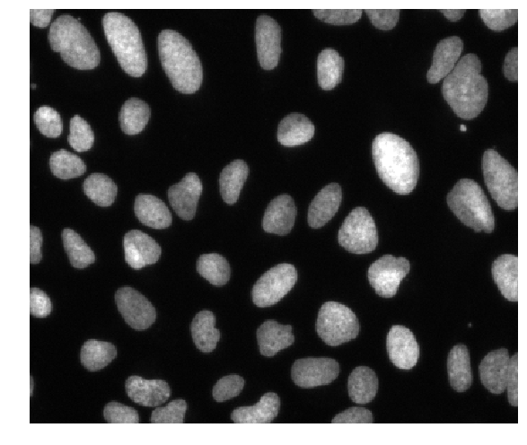
These are fluorescence microscopy images, where we see the nuclei in individual cells.
Step 1: Reading in data
Step one in our image segmentation pipeline is to read in the image data. We can do that with the dask-image imread function.
We pass the path to the folder full of *.tif images from our example data.
from dask_image.imread import imread

images = imread('data/BBBC039/images/*.tif')
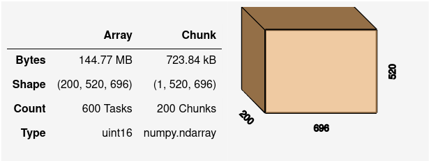
By default, each individual .tif file on disk has become one chunk in our Dask array.
Step 2: Filtering images
Denoising images with a small amount of blur can improve segmentation later on. This is a common first step in a lot of image segmentation pipelines. We can do this with the dask-image gaussian_filter function.
from dask_image import ndfilters

smoothed = ndfilters.gaussian_filter(images, sigma=[0, 1, 1])
Step 3: Segmenting objects
Next, we want to separate the objects in our images from the background. There are lots of different ways we could do this. Because we have fluorescent microscopy images, we’ll use a thresholding method.
Absolute threshold
We could set an absolute threshold value, where we’d consider pixels with intensity values below this threshold to be part of the background.
absolute_threshold = smoothed > 160
Let’s have a look at these images with the napari image viewer. First we’ll need to use the %gui qt magic:
%gui qt
And now we can look a the images with napari:
import napari

viewer = napari.Viewer()
viewer.add_image(absolute_threshold)
viewer.add_image(images, contrast_limits=[0, 2000])
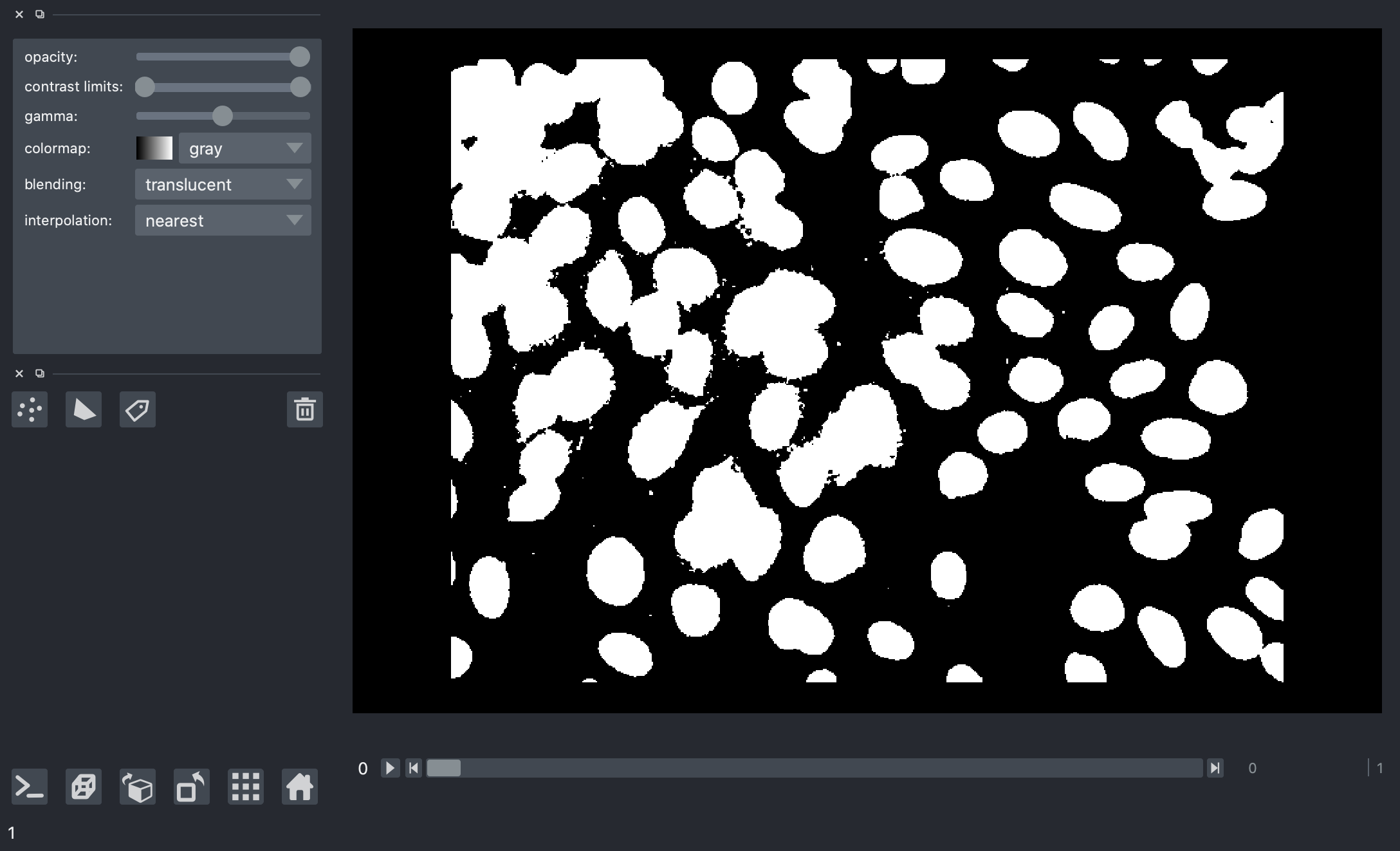
But there’s a problem here.
When we look at the results for different image frames, it becomes clear that there is no “one size fits all” we can use for an absolute threshold value. Some images in the dataset have quite bright backgrounds, others have fluorescent nuclei with low brightness. We’ll have to try a different kind of thresholding method.
Local threshold
We can improve the segmentation using a local thresholding method.
If we calculate a threshold value independently for each image frame then we can avoid the problem caused by fluctuating background intensity between frames.
thresh = ndfilters.threshold_local(smoothed, images.chunksize)
threshold_images = smoothed > thresh
# Let's take a look at the images with napari
viewer.add_image(threshold_images)
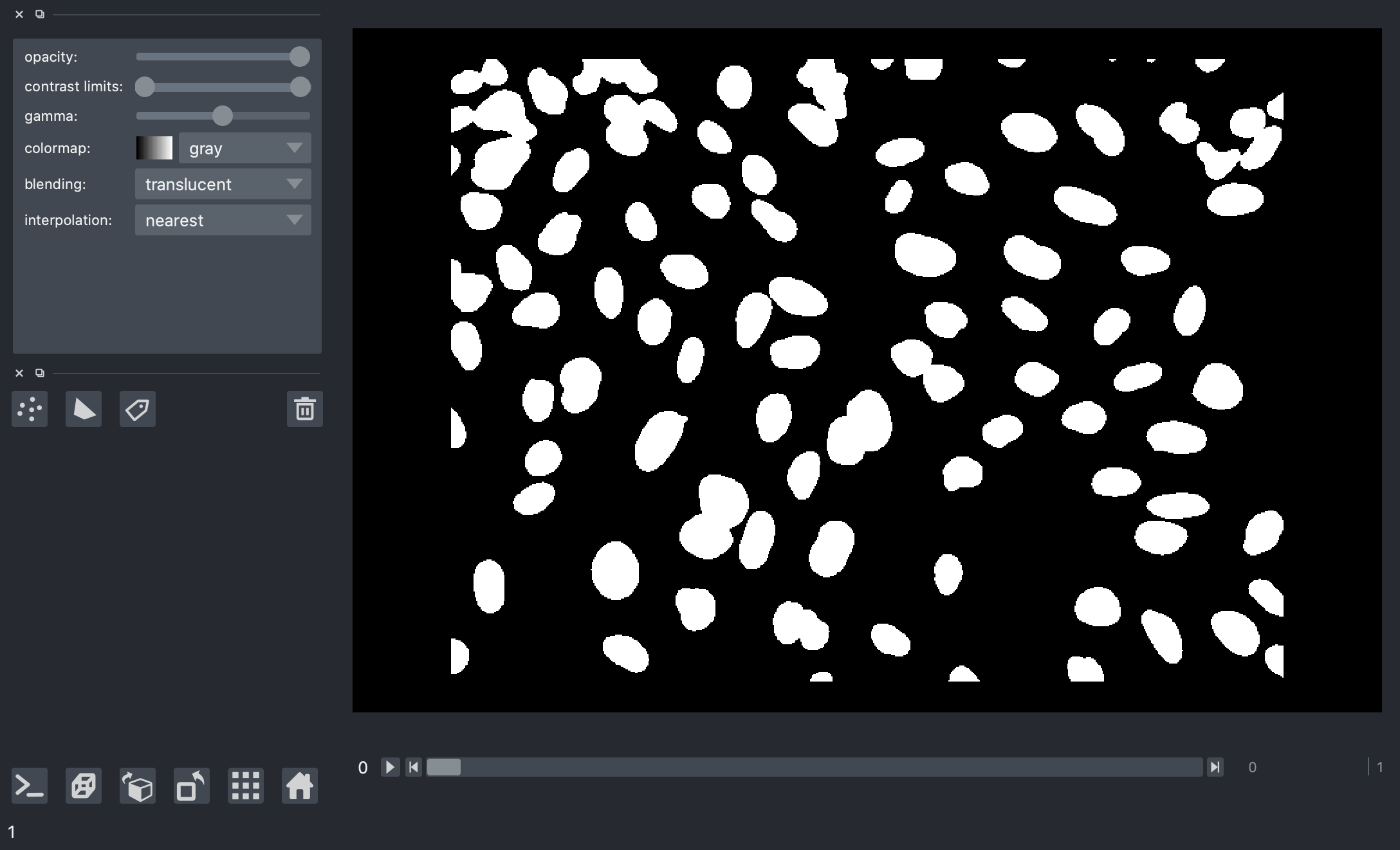
The results here look much better, this is a much cleaner separation of nuclei from the background and it looks good for all the image frames.
Step 4: Morphological operations
Now that we have a binary mask from our threshold, we can clean it up a bit with some morphological operations.
Morphological operations are changes we make to the shape of structures a binary image. We’ll briefly describe some of the basic concepts here, but for a more detailed reference you can look at this excellent page of the OpenCV documentation.
Erosion is an operation where the edges of structures in a binary image are eaten away, or eroded.

Image credit: OpenCV documentation
Dilation is the opposite of an erosion. With dilation, the edges of structures in a binary image are expanded.

Image credit: OpenCV documentation
We can combine morphological operations in different ways to get useful effects.
A morphological opening operation is an erosion, followed by a dilation.

Image credit: OpenCV documentation
In the example image above, we can see the left hand side has a noisy, speckled background. If the structuring element used for the morphological operations is larger than the size of the noisy speckles, they will disappear completely in the first erosion step. Then when it is time to do the second dilation step, there’s nothing left of the noise in the background to dilate. So we have removed the noise in the background, while the major structures we are interested in (in this example, the J shape) are restored almost perfectly.
Let’s use this morphological opening trick to clean up the binary images in our segmentation pipeline.
from dask_image import ndmorph
import numpy as np

structuring_element = np.array([
    [[0, 0, 0], [0, 0, 0], [0, 0, 0]],
    [[0, 1, 0], [1, 1, 1], [0, 1, 0]],
    [[0, 0, 0], [0, 0, 0], [0, 0, 0]]])
binary_images = ndmorph.binary_opening(threshold_images, structure=structuring_element)
You’ll notice here that we need to be a little bit careful about the structuring element. All our image frames are combined in a single Dask array, but we only want to apply the morphological operation independently to each frame. To do this, we sandwich the default 2D structuring element between two layers of zeros. This means the neighbouring image frames have no effect on the result.
# Default 2D structuring element

[[0, 1, 0],
 [1, 1, 1],
 [0, 1, 0]]
Step 5: Measuring objects
The last step in any image processing pipeline is to make some kind of measurement. We’ll turn our binary mask into a label image, and then measure the intensity and size of those objects.
For the sake of keeping the computation time in this tutorial nice and quick, we’ll measure only a small subset of the data. Let’s measure all the objects in the first three image frames (roughly 300 nuclei).
from dask_image import ndmeasure

# Create labelled mask
label_images, num_features = ndmeasure.label(binary_images[:3], structuring_element)
index = np.arange(num_features - 1) + 1  # [1, 2, 3, ...num_features]
Here’s a screenshot of the label image generated from our mask.
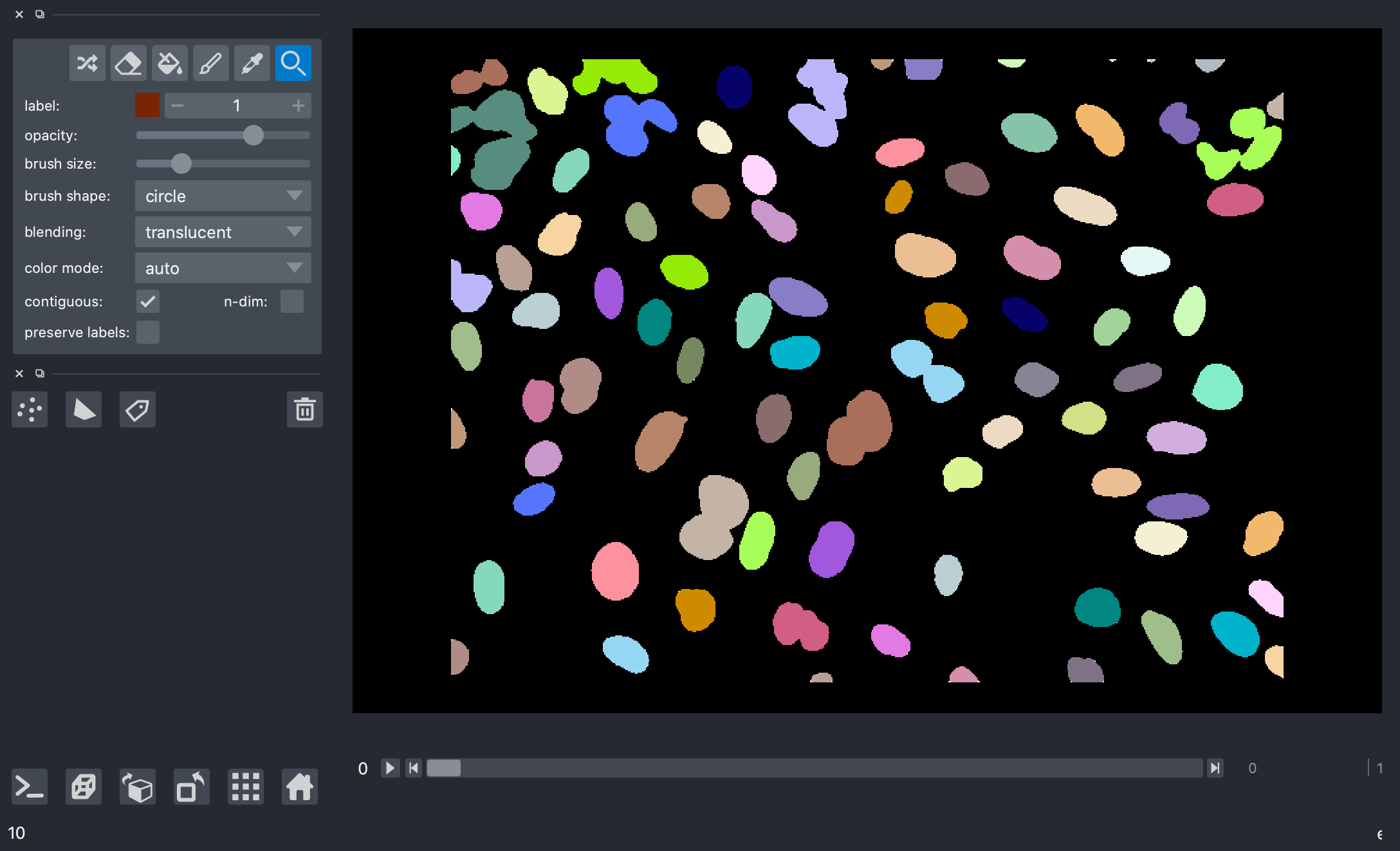
>>> print("Number of nuclei:", num_features.compute())

Number of nuclei: 271
Measure objects in images
The dask-image ndmeasure subpackage includes a number of different measurement functions. In this example, we’ll choose to measure:
- The area in pixels of each object, and
- The average intensity of each object.
area = ndmeasure.area(images[:3], label_images, index)
mean_intensity = ndmeasure.mean(images[:3], label_images, index)
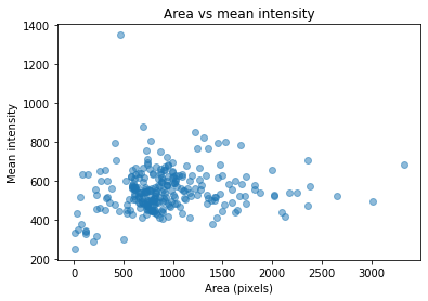
Run computation and plot results
import matplotlib.pyplot as plt

plt.scatter(area, mean_intensity, alpha=0.5)
plt.gca().update(dict(title="Area vs mean intensity", xlabel='Area (pixels)', ylabel='Mean intensity'))
plt.show()
Custom functions
What if you want to do something that isn’t included in the dask-image API? There are several options we can use to write custom functions.
- dask map_overlap / map_blocks
- dask delayed
- scikit-image apply_parallel()
Dask map_overlap and map_blocks
The Dask array map_overlap and map_blocks are what is used to build most of the functions in dask-image. You can use them yourself too. They will apply a function to each chunk in a Dask array.
import dask.array as da

def my_custom_function(args):
    # ... does something really cool

result = da.map_overlap(my_custom_function, my_dask_array, args)
You can read more about overlapping computations here.
Dask delayed
If you want more flexibility and fine-grained control over your computation, then you can use Dask delayed. You can get started with the Dask delayed tutorial here.
scikit-image apply_parallel function
If you’re a person who does a lot of image processing in python, one tool you’re likely to already be using is scikit-image. I’d like to draw your attention to the apply_parallel function available in scikit-image. It uses map-overlap, and can be very helpful.
It’s useful not only when when you have big data, but also in cases where your data fits into memory but the computation you want to apply to the data is memory intensive. This might cause you to exceed the available RAM, and apply_parallel is great for these situations too.
Scaling up computation
When you want to scale up from a laptop onto a supercomputing cluster, you can use dask-distributed to handle that.
from dask.distributed import Client

# Setup a local cluster
# By default this sets up 1 worker per core
client = Client()
client.cluster
See the documentation here to get set up for your system.
Bonus content: using arrays on GPU
We’ve recently been adding GPU support to dask-image.
We’re able to add GPU support using a library called CuPy. CuPy is an array library with a numpy-like API, accelerated with NVIDIA CUDA. Instead of having Dask arrays which contain numpy chunks, we can have Dask arrays containing cupy chunks instead. This blogpost explains the benefits of GPU acceleration and gives some benchmarks for computations on CPU, a single GPU, and multiple GPUs.
GPU support available in dask-image
From dask-image version 0.6.0, there is GPU array support for four of the six subpackages:
- imread
- ndfilters
- ndinterp
- ndmorph
Subpackages of dask-image that do not yet have GPU support are.
- ndfourier
- ndmeasure
We hope to add GPU support to these in the future.
An example
Here’s an example of an image convolution with Dask on the CPU:
# CPU example
import numpy as np
import dask.array as da
from dask_image.ndfilters import convolve

s = (10, 10)
a = da.from_array(np.arange(int(np.prod(s))).reshape(s), chunks=5)
w = np.ones(a.ndim * (3,), dtype=np.float32)
result = convolve(a, w)
result.compute()
And here’s the same example of an image convolution with Dask on the GPU. The only thing necessary to change is the type of input arrays.
# Same example moved to the GPU
import cupy  # <- import cupy instead of numpy (version >=7.7.0)
import dask.array as da
from dask_image.ndfilters import convolve

s = (10, 10)
a = da.from_array(cupy.arange(int(cupy.prod(cupy.array(s)))).reshape(s), chunks=5)  # <- cupy dask array
w = cupy.ones(a.ndim * (3,))  # <- cupy array
result = convolve(a, w)
result.compute()
You can’t mix arrays on the CPU and arrays on the GPU in the same computation. This is why the weights w must be a cupy array in the second example above.
Additionally, you can transfer data between the CPU and GPU. So in situations where the GPU speedup is larger than than cost associated with transferring data, this may be useful to do.
Reading in images onto the GPU
Generally, we want to start our image processing by reading in data from images stored on disk. We can use the imread function with the arraytype=cupy keyword argument to do this.
from dask_image.imread import imread

images = imread('data/BBBC039/images/*.tif')
images_on_gpu = imread('data/BBBC039/images/*.tif', arraytype="cupy")
How you can get involved
Create and share your own segmentation or image processing workflows with Dask (join the current discussion on segmentation or propose a new blogpost topic here)
Contribute to adding GPU support to dask-image: https://github.com/dask/dask-image/issues/133
blog comments powered by Disqus