Image Analysis Redux Dask + CuPy + RL
By John Kirkham (NVIDIA) and Ben Zaitlen (NVIDIA)
Summary
Last year we experimented with Dask/ITK/Scikit-Image to perform large scale image analysis on a stack of 3D images. Specifically, we looked at deconvolution, a common method to deblur images. Now, a year later, we return to these experiments with a better understanding of how Dask and CuPy can interact, enhanced serialization methods, and support from the open-source community. This post looks at the following:
- Implementing a common deconvolution method for CPU + GPU
- Leveraging Dask to perform deconvolution on a larger dataset
- Exploring the results with the Napari image viewer
Image Analysis Redux
Previously we used the Richardson Lucy
(RL)
deconvolution algorithm from ITK and
Scikit-Image.
We left off at theorizing how GPUs could potentially help accelerate these
workflows. Starting with Scikit-Image’s implementation, we naively tried
replacing scipy.signal.convolve calls with cupyx.scipy.ndimage.convolve,
and while performance improved, it did not improve significantly – that is,
we did not get the 100X speed we were looking for.
As it often turns out in mathematics a problem that can be inefficient to solve in one representation can often be made more efficent by transforming the data beforehand. In this new representation we can solve the same problem (convolution in this case) more easily before transforming the result back into a more familiar representation. When it comes to convolution, the transformation we apply is called Fast-Fourier Transform (FFT). Once this is applied we are able to convolve data using a simple multiplication.
As it turns out this FFT transformation is extremely fast on both CPUs and GPUs. Similarly the algorithm we can write with FFTs is accelerated. This is a commonly used technique in the image processing field to speed up convolutions. Despite the added step of doing FFTs, the cost of transformation + the cost of the algorithm is still lower than performing the original algorithm in real space. We (and others before us) found this was the case for Richardson Lucy (on both CPUs and GPUs) and performance continued increasing when we parallelized with Dask over multiple GPUs.
Help from Open-Source
An FFT RL equivalent has been around for some time and the good folks at the Solar Dynamics Observatory built and shared a NumPy/CuPy implementation as part the Atmospheric Imaging Assembly Python package (aiapy). We slightly modified their implementation to handle 3D as well as 2D Point Spread Functions and to take advantage of NEP-18 for convenient dispatching of NumPy and CuPy to NumPy and CuPy functions:
def deconvolve(img, psf=None, iterations=20):
    # Pad PSF with zeros to match image shape
    pad_l, pad_r = np.divmod(np.array(img.shape) - np.array(psf.shape), 2)
    pad_r += pad_l
    psf = np.pad(psf, tuple(zip(pad_l, pad_r)), 'constant', constant_values=0)

    # Recenter PSF at the origin
    # Needed to ensure PSF doesn't introduce an offset when
    # convolving with image
    for i in range(psf.ndim):
        psf = np.roll(psf, psf.shape[i] // 2, axis=i)

    # Convolution requires FFT of the PSF
    psf = np.fft.rfftn(psf)

    # Perform deconvolution in-place on a copy of the image
    # (avoids changing the original)
    img_decon = np.copy(img)
    for _ in range(iterations):
        ratio = img / np.fft.irfftn(np.fft.rfftn(img_decon) * psf)
        img_decon *= np.fft.irfftn((np.fft.rfftn(ratio).conj() * psf).conj())
    return img_decon
For a 1.3 GB image we measured the following:
- CuPy ~3 seconds for 20 iterations
- NumPy ~36 seconds for 2 iterations
We see 10x increase in speed for 10 times the number of iterations – very close to our desired 100x speedup! Let’s explore how this implementation performs with real biological data and Dask…
Define a Dask Cluster and Load the Data
We were provided sample data from Prof. Shroff’s lab at the NIH. The data originally was provided as a 3D TIFF file which we subsequently converted to Zarr with a shape of (950, 2048, 2048).
We start by creating a Dask cluster on a DGX2 (16 GPUs in a single node) and loading the image stored in Zarr :
from dask.distributed import Client
from dask_cuda import LocalCUDACluster
import dask.array as da

import rmm
import cupy as cp

cluster = LocalCUDACluster(
    local_directory="/tmp/bzaitlen",
    enable_nvlink=True,
    rmm_pool_size="26GB",
)
client = Client(cluster)

client.run(
    cp.cuda.set_allocator,
    rmm.rmm_cupy_allocator
)

imgs = da.from_zarr("/public/NVMICROSCOPY/y1z1_C1_A.zarr/")
|
From the Dask output above you can see the data is a z-stack of 950 images
where each slice is 2048x2048. For this data set, we can improve GPU
performance if we operate on larger chunks. Additionally, we need to ensure
the chunks are are least as big as the PSF which in this case is, (128, 128,
128). As we did our work on a DGX2, which has 16 GPUs, we can comfortably fit
the data and perform deconvolution on each GPU if we rechunk the data
accordingly:
# chunk with respect to PSF shape (128, 128, 128)
imgs = imgs.rechunk(chunks={0: 190, 1: 512, 2: 512})
imgs
| Array | Chunk | |
|---|---|---|
| Bytes | 7.97 GB | 99.61 MB |
| Shape | (950, 2048, 2048) | (190, 512, 512) |
| Count | 967 Tasks | 80 Chunks |
| Type | uint16 | numpy.ndarray |
Next, we convert to float32 as the data may not already be of floating point
type. Also 32-bit is a bit faster than 64-bit when computing and saves a bit on
memory. Below we map cupy.asarray onto each block of data. cupy.asarray
moves the data from host memory (NumPy) to the device/GPU (CuPy).
imgs = imgs.astype(np.float32)
c_imgs = imgs.map_blocks(cp.asarray)
|
What we now have is a Dask array composed of 16 CuPy blocks of data. Notice
how Dask provides nice typing information in the SVG output. When we moved
from NumPy to CuPy, the block diagram above displays Type: cupy.ndarray –
this is a nice sanity check.
The last piece we need before running the deconvolution is the PSF which should also be loaded onto the GPU:
import skimage.io

psf = skimage.io.imread("/public/NVMICROSCOPY/PSF.tif")
c_psf = cp.asarray(psf)
Lastly, we call map_overlap with the deconvolve function across the Dask
array:
out = da.map_overlap(
    deconvolve,
    c_imgs,
    psf=c_psf,
    iterations=100,
    meta=c_imgs._meta,
    depth=tuple(np.array(c_psf.shape) // 2),
    boundary="periodic"
)
out
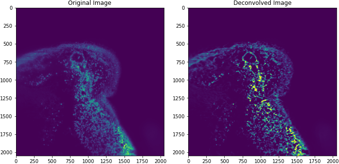
The image above is taken from a mouse intestine.
With Dask and multiple GPUs, we measured deconvolution of an 16GB image in ~30 seconds! But this is just the first step towards accelerated image science.
Napari
Deconvolution is just one operation and one tool, an image scientist or microscopist will need. They will need other tools as they study the underlying biology. Before getting to those next steps, they will need tools to visualize the data. Napari, a multi-dimensional image viewer used in the PyData Bio ecosystem, is a good tool for visualizing this data. As an experiment, we ran the same workflow on a local workstation with 2 Quadro RTX 8000 GPUs connected with NVLink. Example Notebook
By adding a map_blocks call to our array, we can move our data back from
GPU to CPU (device to host).
def cupy_to_numpy(x):
    import cupy as cp
    return cp.asnumpy(x)

np_out = out.map_blocks(cupy_to_numpy, meta=out)
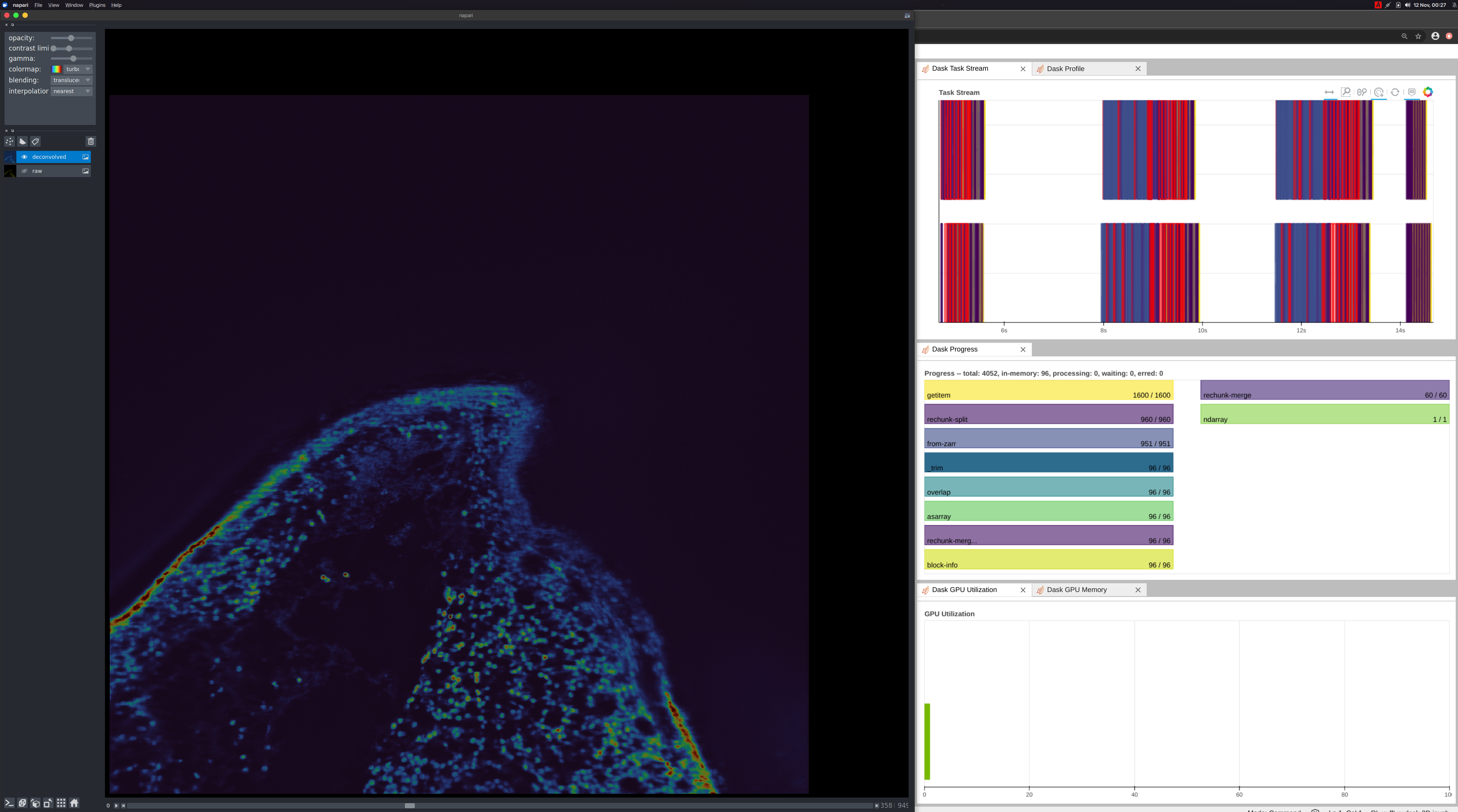
When the user moves the slider on the Napari UI, we are instructing dask to the following:
- Load the data from disk onto the GPU (CuPy)
- Compute the deconvolution
- Move back to the host (NumPy)
- Render with Napari
This has about a second latency which is great for a naive implementation! We
can improve this by adding caching, improving communications with
map_overlap, and optimizing the deconvolution kernel.
Conclusion
We have now shown with Dask + CuPy how one can perform Richardson-Lucy Deconvolution. This required a minimal amount of code. Combining this with an image viewer (Napari), we were able to inspect the data and our result. All of this performed reasonably well by assembling PyData libraries: Dask, CuPy, Zarr, and Napari with a new deconvolution kernel. Hopefully this provides you a good template to get started analyzing your own data and demonstrates the richness and easy expression of custom workflows. If you run into any challenges, please reach out on the Dask issue tracker and we would be happy to engage with you :)
blog comments powered by Disqus