Large SVDs Dask + CuPy + Zarr + Genomics
By Matthew Rocklin (Coiled), Ben Zaitlen (NVIDIA), Alistair Miles (Oxford University)
Summary
We perform Singular Value Decomposition (SVD) calculations on large datasets.
We modify the computation both by using fully precise and approximate methods, and by using both CPUs and GPUs.
In the end we compute an approximate SVD of 200GB of simulated data and using a mutli-GPU machine in 15-20 seconds. Then we run this from a dataset stored in the cloud where we find that I/O is, predictably, a major bottleneck.
SVD - The simple case
Dask arrays contain a relatively sophisticated SVD algorithm that works in the tall-and-skinny or short-and-fat cases, but not so well in the roughly-square case. It works by taking QR decompositions of each block of the array, combining the R matrices, doing another smaller SVD on those, and then performing some matrix multiplication to get back to the full result. It’s numerically stable and decently fast, assuming that the intermediate R matrices of the QR decompositions mostly fit in memory.
The memory constraints here are that if you have an n by m tall and
skinny array (n >> m) cut into k blocks then you need to have about m**2 * k space. This is true in many cases, including typical PCA machine learning
workloads, where you have tabular data with a few columns (hundreds at most)
and many rows.
It’s easy to use and quite robust.
import dask.array as da

x = da.random.random((10000000, 20))
x
|
u, s, v = da.linalg.svd(x)
This works fine in the short and fat case too (when you have far more columns than rows) but we’re always going to assume that one of your dimensions is unchunked, and that the other dimension has chunks that are quite a bit longer, otherwise, things might not fit into memory.
Approximate SVD
If your dataset is large in both dimensions then the algorithm above won’t work as is. However, if you don’t need exact results, or if you only need a few of the components, then there are a number of excellent approximation algorithms.
Dask array has one of these approximation algorithms implemented in the da.linalg.svd_compressed function. And with it we can compute the approximate SVD of very large matrices.
We were recently working on a problem (explained below) and found that we were still running out of memory when dealing with this algorithm. There were two challenges that we ran into:
-
The algorithm requires multiple passes over the data, but the Dask task scheduler was keeping the input matrix in memory after it had been loaded once in order to avoid recomputation. Things still worked, but Dask had to move the data to disk and back repeatedly, which reduced performance significantly.
We resolved this by including explicit recomputation steps in the algorithm.
-
Related chunks of data would be loaded at different times, and so would need to stick around longer than necessary to wait for their associated chunks.
We resolved this by engaging task fusion as an optimization pass.
Before diving further into the technical solution we quickly provide the use case that was motivating this work.
Application - Genomics
Many studies are using genome sequencing to study genetic variation between different individuals within a species. These includes studies of human populations, but also other species such as mice, mosquitoes or disease-causing parasites. These studies will, in general, find a large number of sites in the genome sequence where individuals differ from each other. For example, humans have more than 100 million variable sites in the genome, and modern studies like the UK BioBank are working towards sequencing the genomes of 1 million individuals or more.
In diploid species like humans, mice or mosquitoes, each individual carries two genome sequences, one inherited from each parent. At each of the 100 million variable genome sites there will be two or more “alleles” that a single genome might carry. One way to think about this is via the Punnett square, which represents the different possible genotypes that one individual might carry at one of these variable sites:
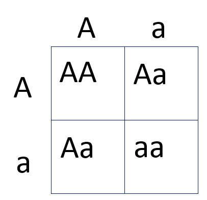
In the above there are three possible genotypes: AA, Aa, and aa. For computational genomics, these genotypes can be encoded as 0, 1, or 2. In a study of a species with M genetic variants assayed in N individual samples, we can represent these genotypes as an (M x N) array of integers. For a modern human genetics study, the scale of this array might approach (100 million x 1 million). (Although in practice, the size of the first dimension (number of variants) can be reduced somewhat, by at least an order of magnitude, because many genetic variants will carry little information and/or be correlated with each other.)
These genetic differences are not random, but carry information about patterns of genetic similarity and shared ancestry between individuals, because of the way they have been inherited through many generations. A common task is to perform a dimensionality reduction analysis on these data, such as a principal components analysis (SVD), to identify genetic structure reflecting these differencies in degree of shared ancestry. This is an essential part of discovering genetic variants associated with different diseases, and for learning more about the genetic history of populations and species.
Reducing the time taken to compute an analysis such as SVD, like all science, allows for exploring larger datasets and testing more hypotheses in less time. Practically, this means not simply a fast SVD but an accelerated pipeline end-to-end, from data loading to analysis, to understanding.
We want to run an experiment in less time than it takes to make a cup of tea
Performant SVDs w/ Dask
Now that we have that scientific background, let’s transition back to talking about computation.
To stop Dask from holding onto the data we intentionally trigger computation as we build up the graph. This is a bit atypical in Dask calculations (we prefer to have as much of the computation at once before computing) but useful given the multiple-pass nature of this problem. This was a fairly easy change, and is available in dask/dask #5041.
Additionally, we found that it was helpful to turn on moderately wide task fusion.
import dask
dask.config.set({"optimization.fuse.ave-width": 5})
Then things work fine
We’re going to try this SVD on a few different choices of hardware including:
- A MacBook Pro
- A DGX-2, an NVIDIA worksation with 16 high-end GPUs and fast interconnect
- A twenty-node cluster on AWS
Macbook Pro
We can happily perform an SVD on a 20GB array on a Macbook Pro
import dask.array as da

x = da.random.random(size=(1_000_000, 20_000), chunks=(20_000, 5_000))

u, s, v = da.linalg.svd_compressed(x, k=10, compute=True)
v.compute()
This call is no longer entirely lazy, and it recomputes x a couple times, but
it works, and it works using only a few GB of RAM on a consumer laptop.
It takes around 2min 30s time to compute that on a laptop. That’s great! It was super easy to try out, didn’t require any special hardware or setup, and in many cases is fast enough. By working locally we can iterate quickly.
Now that things work, we can experiment with different hardware.
Adding GPUs (a 15 second SVD)
Disclaimer: one of the authors (Ben Zaitlen) works for NVIDIA
We can dramatically increase performance by using a multi-GPU machine. NVIDIA and other manufacturers now make machines with multiple GPUs co-located in the same physical box. In the following section, we will run the calculations on a DGX2, a machine with 16 GPUs and fast interconnect between the GPUs.
Below is almost the same code, running in significantly less same time but we make the following changes:
- We increase the size of the array by a factor of 10x
- We switch out NumPy for CuPy, a GPU NumPy implementation
- We use a sixteen-GPU DGX-2 machine with NVLink interconnects between GPUs (NVLink will dramatically decrease transfer time between workers)
On A DGX2 we can calculate an SVD on a 200GB Dask array between 10 to 15 seconds.
The full notebook is here, but the relevant code snippets are below:
# Some GPU specific setup
from dask_cuda import LocalCluster

cluster = LocalCluster(...)
client = Client(cluster)

import cupy
import dask.array as da
rs = da.random.RandomState(RandomState=cupy.random.RandomState)

# Create the data and run the SVD as normal
x = rs.randint(0, 3, size=(10_000_000, 20_000),
               chunks=(20_000, 5_000), dtype="uint8")
x = x.persist()

u, s, v = da.linalg.svd_compressed(x, k=10, seed=rs)
v.compute()
To see this run, we recommend viewing this screencast:
Read dataset from Disk
While impressive, the computation above is mostly bound by generating random data and then performing matrix calculations. GPUs are good at both of these things.
In practice though, our input array won’t be randomly generated, it will be coming from some dataset stored on disk or increasingly more common, stored in the cloud. To make things more realistic we perform a similar calculation with data stored in a Zarr format in GCS
In this Zarr SVD example, we load a 25GB GCS backed data set onto a DGX2, run a few processing steps, then perform an SVD. The combination of preprocessing and SVD calculations ran in 18.7 sec and the data loading took 14.3 seconds.
Again, on a DGX2, from data loading to SVD we are running in time less than it would take to make a cup of tea. However, the data loading can be accelerated. From GCS we are reading into data into the main memory of the machine (host memory), uncompressing the zarr bits, then moving the data from host memory to the GPU (device memory). Passing data back and forth between host and device memory can significantly decrease performance. Reading directly into the GPU, bypassing host memory, would improve the overall pipeline.
And so we come back to a common lesson of high performance computing:
High performance computing isn’t about doing one thing exceedingly well, it’s about doing nothing poorly.
In this case GPUs made our computation fast enough that we now need to focus on other components of our system, notably disk bandwidth, and a direct reader for Zarr data to GPU memory.
Cloud
Diclaimer: one of the authors (Matthew Rocklin) works for Coiled Computing
We can also run this on the cloud with any number of frameworks. In this case we used the Coiled Cloud service to deploy on AWS
from coiled_cloud import Cloud, Cluster
cloud = Cloud()

cloud.create_cluster_type(
    organization="friends",
    name="genomics",
    worker_cpu=4,
    worker_memory="16 GiB",
    worker_environment={
        "OMP_NUM_THREADS": 1,
        "OPENBLAS_NUM_THREADS": 1,
        # "EXTRA_PIP_PACKAGES": "zarr"
    },
)

cluster = Cluster(
    organization="friends",
    typename="genomics",
    n_workers=20,
)

from dask.distributed import Client
client = Client(cluster)

# then proceed as normal
Using 20 machines with a total of 80 CPU cores on a dataset that was 10x larger than the MacBook pro example we were able to run in about the same amount of time. This shows near optimal scaling for this problem, which is nice to see given how complex the SVD calculation is.
A screencast of this problem is viewable here
Compression
One of the easiest ways for us to improve performance is to reduce the size of this data through compression. This data is highly compressible for two reasons:
- The real-world data itself has structure and repetition (although the random play data does not)
- We’re storing entries that take on only four values. We’re using eight-bit integers when we only needed two-bit integers
Let’s solve the second problem first.
Compression with bit twiddling
Ideally Numpy would have a two-bit integer datatype. Unfortunately it doesn’t, and this is hard because memory in computers is generally thought of in full bytes.
To work around this we can use bit arithmetic to shove four values into a single value Here are functions that do that, assuming that our array is square, and the last dimension is divisible by four.
import numpy as np

def compress(x: np.ndarray) -> np.ndarray:
    out = np.zeros_like(x, shape=(x.shape[0], x.shape[1] // 4))
    out += x[:, 0::4]
    out += x[:, 1::4] << 2
    out += x[:, 2::4] << 4
    out += x[:, 3::4] << 6
    return out


def decompress(out: np.ndarray) -> np.ndarray:
    back = np.zeros_like(out, shape=(out.shape[0], out.shape[1] * 4))
    back[:, 0::4] = out & 0b00000011
    back[:, 1::4] = (out & 0b00001100) >> 2
    back[:, 2::4] = (out & 0b00110000) >> 4
    back[:, 3::4] = (out & 0b11000000) >> 6
    return back
Then, we can use these functions along with Dask to store our data in a compressed state, but lazily decompress on-demand.
x = x.map_blocks(compress).persist().map_blocks(decompress)
That’s it. We compress each block our data and store that in memory.
However the output variable that we have, x will decompress each chunk before
we operate on it, so we don’t need to worry about handling compressed blocks.
Compression with Zarr
A slightly more general but probably less efficient route would be to compress our arrays with a proper compression library like Zarr.
The example below shows how we do this in practice.
import zarr
import numpy as np
from numcodecs import Blosc
compressor = Blosc(cname='lz4', clevel=3, shuffle=Blosc.BITSHUFFLE)


x = x.map_blocks(zarr.array, compressor=compressor).persist().map_blocks(np.array)
Additionally, if we’re using the dask-distributed scheduler then we want to make sure that the Blosc compression library doesn’t use additional threads. That way we don’t have parallel calls of a parallel library, which can cause some contention
def set_no_threads_blosc():
    """ Stop blosc from using multiple threads """
    import numcodecs
    numcodecs.blosc.use_threads = False

# Run on all workers
client.register_worker_plugin(set_no_threads_blosc)
This approach is more general, and probably a good trick to have up ones’ sleeve, but it also doesn’t work on GPUs, which in the end is why we ended up going with the bit-twiddling approach one section above, which uses API that was uniformly accessible within the Numpy and CuPy libraries.
Final Thoughts
In this post we did a few things, all around a single important problems in genomics.
- We learned a bit of science
- We translated a science problem into a computational problem, and in particular into a request to perform large singular value decompositions
- We used a canned algorithm in dask.array that performed pretty well, assuming that we’re comfortable going over the array in a few passes
- We then tried that algorithm on three architectures quickly
- A Macbook Pro
- A multi-GPU machine
- A cluster in the cloud
- Finally we talked about some tricks to pack more data into the same memory with compression
This problem was nice in that we got to dive deep into a technical science problem, and yet also try a bunch of architecture quickly to investigate hardware choices that we might make in the future.
We used several technologies here today, made by several different communities and companies. It was great to see how they all worked together seamlessly to provide a flexible-yet-consistent experience.
blog comments powered by Disqus