DataFrame Groupby Aggregations deepdive on groupbys
By Benjamin Zaitlen & James Bourbeau
Groupby Aggregations with Dask
In this post we’ll dive into how Dask computes groupby aggregations. These are commonly used operations for ETL and analysis in which we split data into groups, apply a function to each group independently, and then combine the results back together. In the PyData/R world this is often referred to as the split-apply-combine strategy (first coined by Hadley Wickham) and is used widely throughout the Pandas ecosystem.
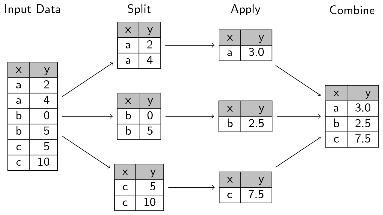
Image courtesy of swcarpentry.github.io
Dask leverages this idea using a similarly catchy name: apply-concat-apply or aca for short. Here we’ll explore the aca strategy in both simple and complex operations.
First, recall that a Dask DataFrame is a collection of DataFrame objects (e.g. each partition of a Dask DataFrame is a Pandas DataFrame). For example, let’s say we have the following Pandas DataFrame:
>>> import pandas as pd
>>> df = pd.DataFrame(dict(a=[1, 1, 2, 3, 3, 1, 1, 2, 3, 3, 99, 10, 1],
...                        b=[1, 3, 10, 3, 2, 1, 3, 10, 3, 3, 12, 0, 9],
...                        c=[2, 4, 5, 2, 3, 5, 2, 3, 9, 2, 44, 33, 2]))
>>> df
     a   b   c
0    1   1   2
1    1   3   4
2    2  10   5
3    3   3   2
4    3   2   3
5    1   1   5
6    1   3   2
7    2  10   3
8    3   3   9
9    3   3   2
10  99  12  44
11  10   0  33
12   1   9   2
To create a Dask DataFrame with three partitions from this data, we could partition df between the indices of: (0, 4), (5, 9), and (10, 12). We can perform this partitioning with Dask by using the from_pandas function with npartitions=3:
>>> import dask.dataframe as dd
>>> ddf = dd.from_pandas(df, npartitions=3)
The 3 partitions are simply 3 individual Pandas DataFrames:
>>> ddf.partitions[0].compute()
   a   b  c
0  1   1  2
1  1   3  4
2  2  10  5
3  3   3  2
4  3   2  3
Apply-concat-apply
When Dask applies a function and/or algorithm (e.g. sum, mean, etc.) to a Dask DataFrame, it does so by applying that operation to all the constituent partitions independently, collecting (or concatenating) the outputs into intermediary results, and then applying the operation again to the intermediary results to produce a final result. Internally, Dask re-uses the same apply-concat-apply methodology for many of its internal DataFrame calculations.
Let’s break down how Dask computes ddf.groupby(['a', 'b']).c.sum() by going through each step in the aca process. We’ll begin by splitting our df Pandas DataFrame into three partitions:
>>> df_1 = df[:5]
>>> df_2 = df[5:10]
>>> df_3 = df[-3:]
Apply
Next we perform the same groupby(['a', 'b']).c.sum() operation on each of our three partitions:
>>> sr1 = df_1.groupby(['a', 'b']).c.sum()
>>> sr2 = df_2.groupby(['a', 'b']).c.sum()
>>> sr3 = df_3.groupby(['a', 'b']).c.sum()
These operations each produce a Series with a MultiIndex:
>>> sr1
a  b
1  1     2
   3     4
2  10    5
3  2     3
   3     2
Name: c, dtype: int64
|
>>> sr2
a  b
1  1      5
   3      2
2  10     3
3  3     11
Name: c, dtype: int64
|
>>> sr3
a   b
1   9      2
10  0     33
99  12    44
Name: c, dtype: int64
|
|---|
The conCat!
After the first apply, the next step is to concatenate the intermediate sr1, sr2, and sr3 results. This is fairly straightforward to do using the Pandas concat function:
>>> sr_concat = pd.concat([sr1, sr2, sr3])
>>> sr_concat
a   b
1   1      2
    3      4
2   10     5
3   2      3
    3      2
1   1      5
    3      2
2   10     3
3   3     11
1   9      2
10  0     33
99  12    44
Name: c, dtype: int64
Apply Redux
Our final step is to apply the same groupby(['a', 'b']).c.sum() operation again on the concatenated sr_concat Series. However we no longer have columns a and b, so how should we proceed?
Zooming out a bit, our goal is to add the values in the column which have the same index. For example, there are two rows with the index (1, 1) with corresponding values: 2, 5. So how can we groupby the indices with the same value? A MutliIndex uses levels to define what the value is at a give index. Dask determines and uses these levels in the final apply step of the apply-concat-apply calculation. In our case, the level is [0, 1], that is, we want both the index at the 0th level and the 1st level and if we group by both, 0, 1, we will have effectively grouped the same indices together:
>>> total = sr_concat.groupby(level=[0, 1]).sum()
>>> total
a   b
1   1      7
    3      6
    9      2
2   10     8
3   2      3
    3     13
10  0     33
99  12    44
Name: c, dtype: int64
|
>>> ddf.groupby(['a', 'b']).c.sum().compute()
a   b
1   1      7
    3      6
2   10     8
3   2      3
    3     13
1   9      2
10  0     33
99  12    44
Name: c, dtype: int64
|
>>> df.groupby(['a', 'b']).c.sum()
a   b
1   1      7
    3      6
    9      2
2   10     8
3   2      3
    3     13
10  0     33
99  12    44
Name: c, dtype: int64
|
|---|
Additionally, we can easily examine the steps of this apply-concat-apply calculation by visualizing the task graph for the computation:
>>> ddf.groupby(['a', 'b']).c.sum().visualize()

sum is rather a straight-forward calculation. What about something a bit more complex like mean?
>>> ddf.groupby(['a', 'b']).c.mean().visualize()

Mean is a good example of an operation which doesn’t directly fit in the aca model – concatenating mean values and taking the mean again will yield incorrect results. Like any style of computation: vectorization, Map/Reduce, etc., we sometime need to creatively fit the computation to the style/mode. In the case of aca we can often break down the calculation into constituent parts. For mean, this would be sum and count:
From the task graph above, we can see that two independent tasks for each partition: series-groupby-count-chunk and series-groupby-sum-chunk. The results are then aggregated into two final nodes: series-groupby-count-agg and series-groupby-sum-agg and then we finally calculate the mean: total sum / total count.
blog comments powered by Disqus