Dask Release 0.14.3
This work is supported by Continuum Analytics and the Data Driven Discovery Initiative from the Moore Foundation.
I’m pleased to announce the release of Dask version 0.14.3. This release contains a variety of performance and feature improvements. This blogpost includes some notable features and changes since the last release on March 22nd.
As always you can conda install from conda-forge
conda install -c conda-forge dask distributed
or you can pip install from PyPI
pip install dask[complete] --upgrade
Conda packages should be on the default channel within a few days.
Arrays
Sparse Arrays
Dask.arrays now support sparse arrays and mixed dense/sparse arrays.
>>> import dask.array as da

>>> x = da.random.random(size=(10000, 10000, 10000, 10000),
...                      chunks=(100, 100, 100, 100))
>>> x[x < 0.99] = 0

>>> import sparse
>>> s = x.map_blocks(sparse.COO)  # parallel array of sparse arrays
In order to support sparse arrays we did two things:
- Made dask.array support ndarray containers other than NumPy, as long as they were API compatible
- Made a small sparse array library that was API compatible to the numpy.ndarray
This process was pretty easy and could be extended to other systems.
This also allows for different kinds of ndarrays in the same Dask array, as
long as interactions between the arrays are well defined (using the standard
NumPy protocols like __array_priority__ and so on.)
Documentation: http://dask.pydata.org/en/latest/array-sparse.html
Update: there is already a pull request for Masked arrays
Reworked FFT code
The da.fft submodule has been extended to include most of the functions in
np.fft, with the caveat that multi-dimensional FFTs will only work along
single-chunk dimensions. Still, given that rechunking is decently fast today
this can be very useful for large image stacks.
Documentation: http://dask.pydata.org/en/latest/array-api.html#fast-fourier-transforms
Constructor Plugins
You can now run arbitrary code whenever a dask array is constructed. This empowers users to build in their own policies like rechunking, warning users, or eager evaluation. A dask.array plugin takes in a dask.array and returns either a new dask array, or returns None, in which case the original will be returned.
>>> def f(x):
...     print('%d bytes' % x.nbytes)

>>> with dask.set_options(array_plugins=[f]):
...     x = da.ones((10, 1), chunks=(5, 1))
...     y = x.dot(x.T)
80 bytes
80 bytes
800 bytes
800 bytes
This can be used, for example, to convert dask.array code into numpy code to identify bugs quickly:
>>> with dask.set_options(array_plugins=[lambda x: x.compute()]):
...     x = da.arange(5, chunks=2)

>>> x  # this was automatically converted into a numpy array
array([0, 1, 2, 3, 4])
Or to warn users if they accidentally produce an array with large chunks:
def warn_on_large_chunks(x):
    shapes = list(itertools.product(*x.chunks))
    nbytes = [x.dtype.itemsize * np.prod(shape) for shape in shapes]
    if any(nb > 1e9 for nb in nbytes):
        warnings.warn("Array contains very large chunks")

with dask.set_options(array_plugins=[warn_on_large_chunks]):
    ...
These features were heavily requested by the climate science community, which tends to serve both highly technical computer scientists, and less technical climate scientists who were running into issues with the nuances of chunking.
DataFrames
Dask.dataframe changes are both numerous, and very small, making it difficult to give a representative accounting of recent changes within a blogpost. Typically these include small changes to either track new Pandas development, or to fix slight inconsistencies in corner cases (of which there are many.)
Still, two highlights follow:
Rolling windows with time intervals
>>> s.rolling('2s').count().compute()
2017-01-01 00:00:00    1.0
2017-01-01 00:00:01    2.0
2017-01-01 00:00:02    2.0
2017-01-01 00:00:03    2.0
2017-01-01 00:00:04    2.0
2017-01-01 00:00:05    2.0
2017-01-01 00:00:06    2.0
2017-01-01 00:00:07    2.0
2017-01-01 00:00:08    2.0
2017-01-01 00:00:09    2.0
dtype: float64
Read Parquet data with Arrow
Dask now supports reading Parquet data with both fastparquet (a Numpy/Numba solution) and Arrow and Parquet-CPP.
df = dd.read_parquet('/path/to/mydata.parquet', engine='fastparquet')
df = dd.read_parquet('/path/to/mydata.parquet', engine='arrow')
Hopefully this capability increases the use of both projects and results in greater feedback to those libraries so that they can continue to advance Python’s access to the Parquet format.
Graph Optimizations
Dask performs a few passes of simple linear-time graph optimizations before sending a task graph to the scheduler. These optimizations currently vary by collection type, for example dask.arrays have different optimizations than dask.dataframes. These optimizations can greatly improve performance in some cases, but can also increase overhead, which becomes very important for large graphs.
As Dask has grown into more communities, each with strong and differing performance constraints, we’ve found that we needed to allow each community to define its own optimization schemes. The defaults have not changed, but now you can override them with your own. This can be set globally or with a context manager.
def my_optimize_function(graph, keys):
    """ Takes a task graph and a list of output keys, returns new graph """
    new_graph = {...}
    return new_graph

with dask.set_options(array_optimize=my_optimize_function,
                      dataframe_optimize=None,
                      delayed_optimize=my_other_optimize_function):
    x, y = dask.compute(x, y)
Documentation: http://dask.pydata.org/en/latest/optimize.html#customizing-optimization
Speed improvements
Additionally, task fusion has been significantly accelerated. This is very important for large graphs, particularly in dask.array computations.
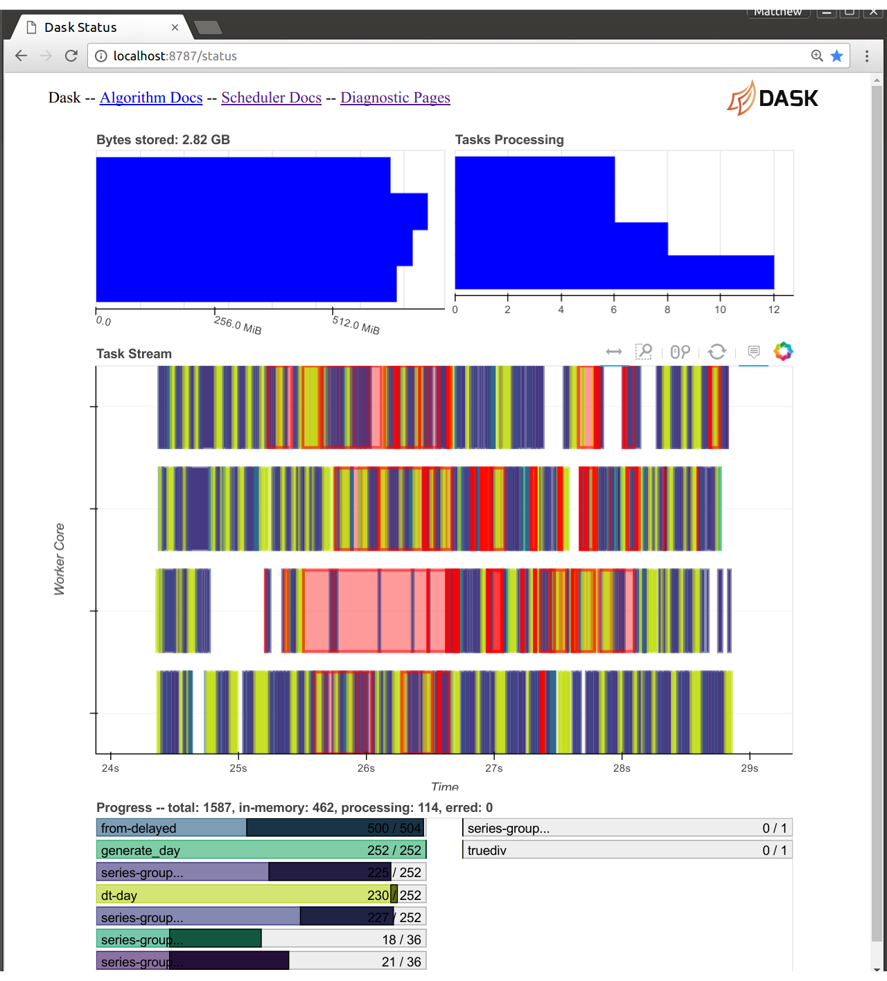
Web Diagnostics
The distributed scheduler’s web diagnostic page is now served from within the dask scheduler process. This is both good and bad:
- Good: It is much easier to make new visuals
- Bad: Dask and Bokeh now share a single CPU
Because Bokeh and Dask now share the same Tornado event loop we no longer need to send messages between them to then send out to a web browser. The Bokeh server has full access to all of the scheduler state. This lets us build new diagnostic pages more easily. This has been around for a while but was largely used for development. In this version we’ve switched the new version to be default and turned off the old one.
The cost here is that the Bokeh scheduler can take 10-20% of the CPU use. If you are running a computation that heavily taxes the scheduler then you might want to close your diagnostic pages. Fortunately, this almost never happens. The dask scheduler is typically fast enough to never get close to this limit.
Tornado difficulties
Beware that the current versions of Bokeh (0.12.5) and Tornado (4.5) do not play well together. This has been fixed in development versions, and installing with conda is fine, but if you naively pip install then you may experience bad behavior.
Joblib
The Dask.distributed Joblib backend now includes a scatter= keyword, allowing
you to pre-scatter select variables out to all of the Dask workers. This
significantly cuts down on overhead, especially on machine learning workloads
where most of the data doesn’t change very much.
# Send the training data only once to each worker
with parallel_backend('dask.distributed', scheduler_host='localhost:8786',
                      scatter=[digits.data, digits.target]):
    search.fit(digits.data, digits.target)
Early trials indicate that computations like scikit-learn’s RandomForest scale nicely on a cluster without any additional code.
Documentation: http://distributed.readthedocs.io/en/latest/joblib.html
Preload scripts
When starting a dask.distributed scheduler or worker people often want to include a bit of custom setup code, for example to configure loggers, authenticate with some network system, and so on. This has always been possible if you start scheduler and workers from within Python but is tricky if you want to use the command line interface. Now you can write your custom code as a separate standalone script and ask the command line interface to run it for you at startup:
# scheduler-setup.py
from distributed.diagnostics.plugin import SchedulerPlugin

class MyPlugin(SchedulerPlugin):
    """ Prints a message whenever a worker is added to the cluster """
    def add_worker(self, scheduler=None, worker=None, **kwargs):
        print("Added a new worker at", worker)

    def dask_setup(scheduler):
        plugin = MyPlugin()
        scheduler.add_plugin(plugin)
dask-scheduler --preload scheduler-setup.py
This makes it easier for people to adapt Dask to their particular institution.
Documentation: http://distributed.readthedocs.io/en/latest/setup.html#customizing-initialization
Network Interfaces (for infiniband)
Many people use Dask on high performance supercomputers. This hardware differs from typical commodity clusters or cloud services in several ways, including very high performance network interconnects like InfiniBand. Typically these systems also have normal ethernet and other networks. You’re probably familiar with this on your own laptop when you have both ethernet and wireless:
$ ifconfig
lo          Link encap:Local Loopback                       # Localhost
            inet addr:127.0.0.1  Mask:255.0.0.0
            inet6 addr: ::1/128 Scope:Host
eth0        Link encap:Ethernet  HWaddr XX:XX:XX:XX:XX:XX   # Ethernet
            inet addr:192.168.0.101
            ...
ib0         Link encap:Infiniband                           # Fast InfiniBand
            inet addr:172.42.0.101
The default systems Dask uses to determine network interfaces often choose
ethernet by default. If you are on an HPC system then this is likely not
optimal. You can direct Dask to choose a particular network interface with the
--interface keyword
$ dask-scheduler --interface ib0
distributed.scheduler - INFO -   Scheduler at: tcp://172.42.0.101:8786

$ dask-worker tcp://172.42.0.101:8786 --interface ib0
Efficient as_completed
The as_completed iterator returns futures in the order in which they complete. It is the base of many asynchronous applications using Dask.
>>> x, y, z = client.map(inc, [0, 1, 2])
>>> for future in as_completed([x, y, z]):
...     print(future.result())
2
0
1
It can now also wait to yield an element only after the result also arrives
>>> for future, result in as_completed([x, y, z], with_results=True):
...     print(result)
2
0
1
And also yield all futures (and results) that have finished up until this point.
>>> for futures in as_completed([x, y, z]).batches():
...    print(client.gather(futures))
(2, 0)
(1,)
Both of these help to decrease the overhead of tight inner loops within asynchronous applications.
Example blogpost here: /2017/04/19/dask-glm-2
Co-released libraries
This release is aligned with a number of other related libraries, notably Pandas, and several smaller libraries for accessing data, including s3fs, hdfs3, fastparquet, and python-snappy each of which have seen numerous updates over the past few months. Much of the work of these latter libraries is being coordinated by Martin Durant
Acknowledgements
The following people contributed to the dask/dask repository since the 0.14.1 release on March 22nd
- Antoine Pitrou
- Dmitry Shachnev
- Erik Welch
- Eugene Pakhomov
- Jeff Reback
- Jim Crist
- John A Kirkham
- Joris Van den Bossche
- Martin Durant
- Matthew Rocklin
- Michal Ficek
- Noah D Brenowitz
- Stuart Archibald
- Tom Augspurger
- Wes McKinney
- wikiped
The following people contributed to the dask/distributed repository since the 1.16.1 release on March 22nd
- Antoine Pitrou
- Bartosz Marcinkowski
- Ben Schreck
- Jim Crist
- Jens Nie
- Krisztián Szűcs
- Lezyes
- Luke Canavan
- Martin Durant
- Matthew Rocklin
- Phil Elson
blog comments powered by Disqus