Write Complex Parallel Algorithms Fancy graphs, Mathematicians, and SVD
This work is supported by Continuum Analytics and the XDATA Program as part of the Blaze Project
tl;dr: We discuss the use of complex dask graphs for non-trivial algorithms. We show off an on-disk parallel SVD.
Most Parallel Computation is Simple
Most parallel workloads today are fairly trivial:
>>> import dask.bag as db
>>> b = db.from_s3('githubarchive-data', '2015-01-01-*.json.gz')
          .map(json.loads)
          .map(lambda d: d['type'] == 'PushEvent')
          .count()
Graphs for these computations look like the following:
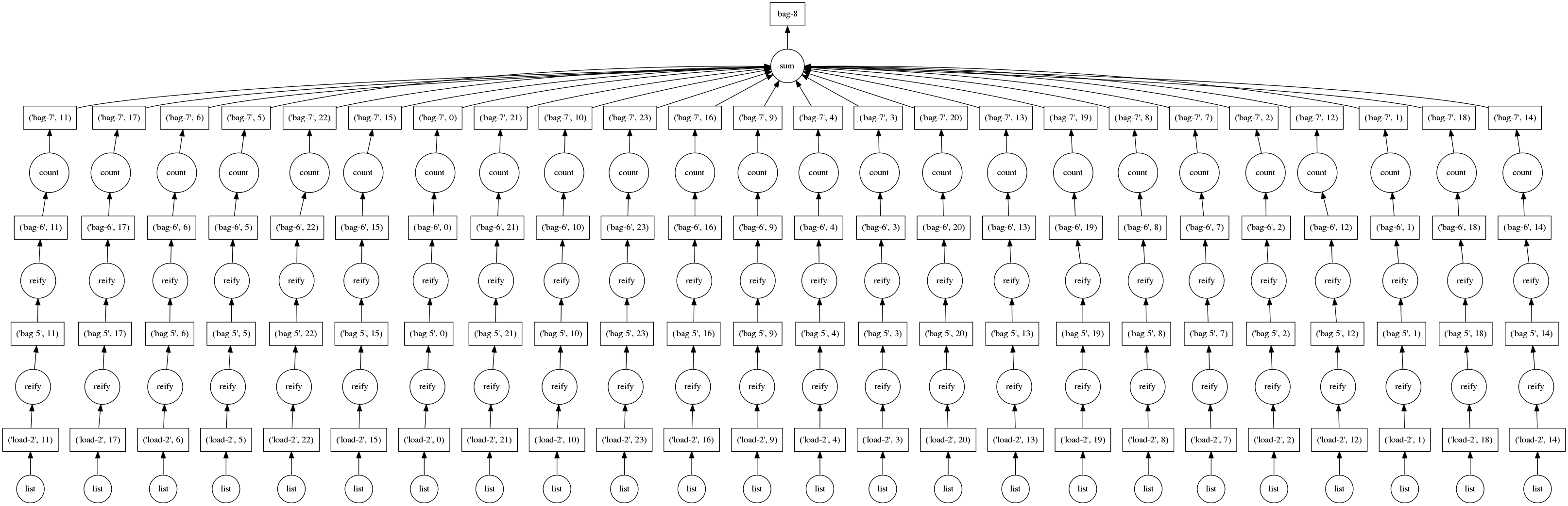
This is great; these are simple problems to solve efficiently in parallel. Generally these simple computations occur at the beginning of our analyses.
Sophisticated Algorithms can be Complex
Later in our analyses we want more complex algorithms for statistics
, machine learning, etc.. Often this stage fits
comfortably in memory, so we don’t worry about parallelism and can use
statsmodels or scikit-learn on the gigabyte result we’ve gleaned from
terabytes of data.
However, if our reduced result is still large then we need to think about sophisticated parallel algorithms. This is fresh space with lots of exciting academic and software work.
Example: Parallel, Stable, Out-of-Core SVD
I’d like to show off work by Mariano Tepper,
who is responsible for dask.array.linalg. In particular he has a couple of
wonderful algorithms for the
Singular Value Decomposition (SVD)
(also strongly related to Principal Components Analysis (PCA).)
Really I just want to show off this pretty graph.
>>> import dask.array as da
>>> x = da.ones((5000, 1000), chunks=(1000, 1000))
>>> u, s, v = da.linalg.svd(x)
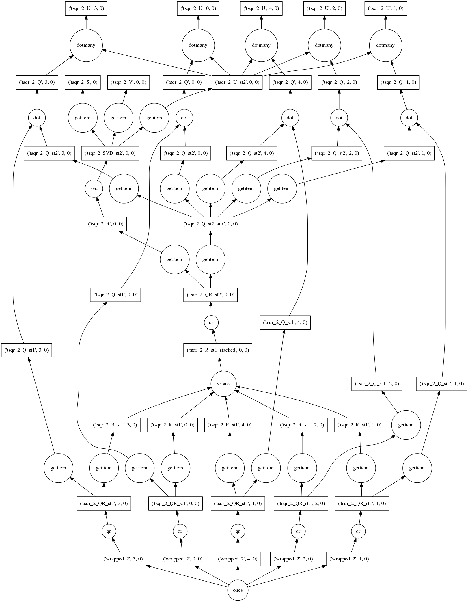
This algorithm computes the exact SVD (up to numerical precision) of a large
tall-and-skinny matrix in parallel in many small chunks. This allows it to
operate out-of-core (from disk) and use multiple cores in parallel. At the
bottom we see the construction of our trivial array of ones, followed by many
calls to np.linalg.qr on each of the blocks. Then there is a lot of
rearranging of various pieces as they are stacked, multiplied, and undergo more
rounds of np.linalg.qr and np.linalg.svd. The resulting arrays are
available in many chunks at the top and second-from-top rows.
The dask dict for one of these
arrays, s, looks like the following:
>>> s.dask
{('x', 0, 0): (np.ones, (1000, 1000)),
 ('x', 1, 0): (np.ones, (1000, 1000)),
 ('x', 2, 0): (np.ones, (1000, 1000)),
 ('x', 3, 0): (np.ones, (1000, 1000)),
 ('x', 4, 0): (np.ones, (1000, 1000)),
 ('tsqr_2_QR_st1', 0, 0): (np.linalg.qr, ('x', 0, 0)),
 ('tsqr_2_QR_st1', 1, 0): (np.linalg.qr, ('x', 1, 0)),
 ('tsqr_2_QR_st1', 2, 0): (np.linalg.qr, ('x', 2, 0)),
 ('tsqr_2_QR_st1', 3, 0): (np.linalg.qr, ('x', 3, 0)),
 ('tsqr_2_QR_st1', 4, 0): (np.linalg.qr, ('x', 4, 0)),
 ('tsqr_2_R', 0, 0): (operator.getitem, ('tsqr_2_QR_st2', 0, 0), 1),
 ('tsqr_2_R_st1', 0, 0): (operator.getitem,('tsqr_2_QR_st1', 0, 0), 1),
 ('tsqr_2_R_st1', 1, 0): (operator.getitem, ('tsqr_2_QR_st1', 1, 0), 1),
 ('tsqr_2_R_st1', 2, 0): (operator.getitem, ('tsqr_2_QR_st1', 2, 0), 1),
 ('tsqr_2_R_st1', 3, 0): (operator.getitem, ('tsqr_2_QR_st1', 3, 0), 1),
 ('tsqr_2_R_st1', 4, 0): (operator.getitem, ('tsqr_2_QR_st1', 4, 0), 1),
 ('tsqr_2_R_st1_stacked', 0, 0): (np.vstack,
                                   [('tsqr_2_R_st1', 0, 0),
                                    ('tsqr_2_R_st1', 1, 0),
                                    ('tsqr_2_R_st1', 2, 0),
                                    ('tsqr_2_R_st1', 3, 0),
                                    ('tsqr_2_R_st1', 4, 0)])),
 ('tsqr_2_QR_st2', 0, 0): (np.linalg.qr, ('tsqr_2_R_st1_stacked', 0, 0)),
 ('tsqr_2_SVD_st2', 0, 0): (np.linalg.svd, ('tsqr_2_R', 0, 0)),
 ('tsqr_2_S', 0): (operator.getitem, ('tsqr_2_SVD_st2', 0, 0), 1)}
So to write complex parallel algorithms we write down dictionaries of tuples of functions.
The dask schedulers take care of executing this graph in parallel using multiple threads. Here is a profile result of a larger computation on a 30000x1000 array:
Low Barrier to Entry
Looking at this graph you may think “Wow, Mariano is awesome” and indeed he is. However, he is more an expert at linear algebra than at Python programming. Dask graphs (just dictionaries) are simple enough that a domain expert was able to look at them say “Yeah, I can do that” and write down the very complex algorithms associated to his domain, leaving the execution of those algorithms up to the dask schedulers.
You can see the source code that generates the above graphs on GitHub.
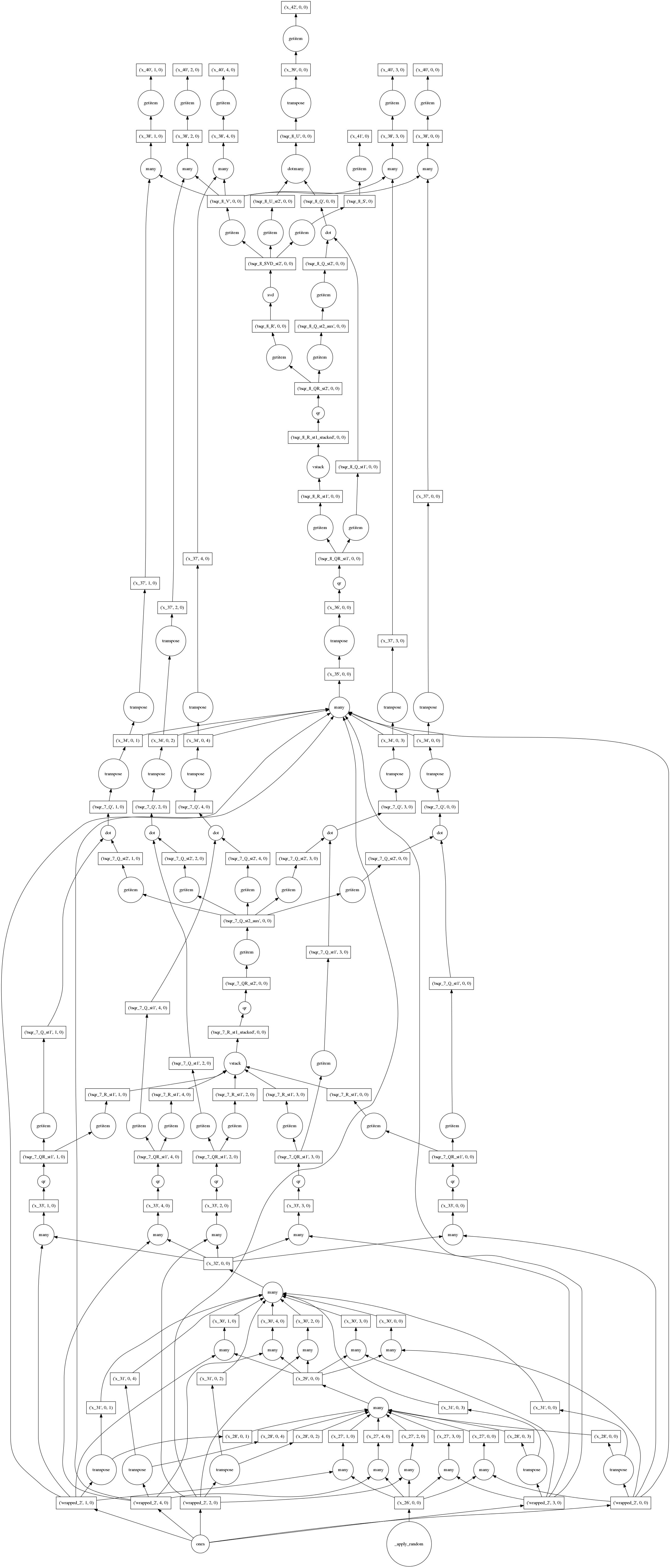
Randomized Parallel Out-of-Core SVD
A few weeks ago a genomics researcher asked for an approximate/randomized variant to SVD. Mariano had a solution up in a few days.
>>> import dask.array as da
>>> x = da.ones((5000, 1000), chunks=(1000, 1000))
>>> u, s, v = da.linalg.svd_compressed(x, k=100, n_power_iter=2)
I’ll omit the full dict for obvious space reasons.
Final Thoughts
Dask graphs let us express parallel algorithms with very little extra complexity. There are no special objects or frameworks to learn, just dictionaries of tuples of functions. This allows domain experts to write sophisticated algorithms without fancy code getting in their way.
blog comments powered by Disqus